2.1. Introduction
Tkwant is a Python package for the simulation of quantum nanoelectronics devices on which external time-dependent perturbations are applied. Tkwant is an extension of the Kwant package and can handle the same types of systems: discrete tight-binding like models that consist of an arbitrary central region connected to semi-infinite electrodes, also called leads. For such systems, tkwant provides algorithms to simulate the time-evolution of manybody expectation values, as e.g. densities and currents.
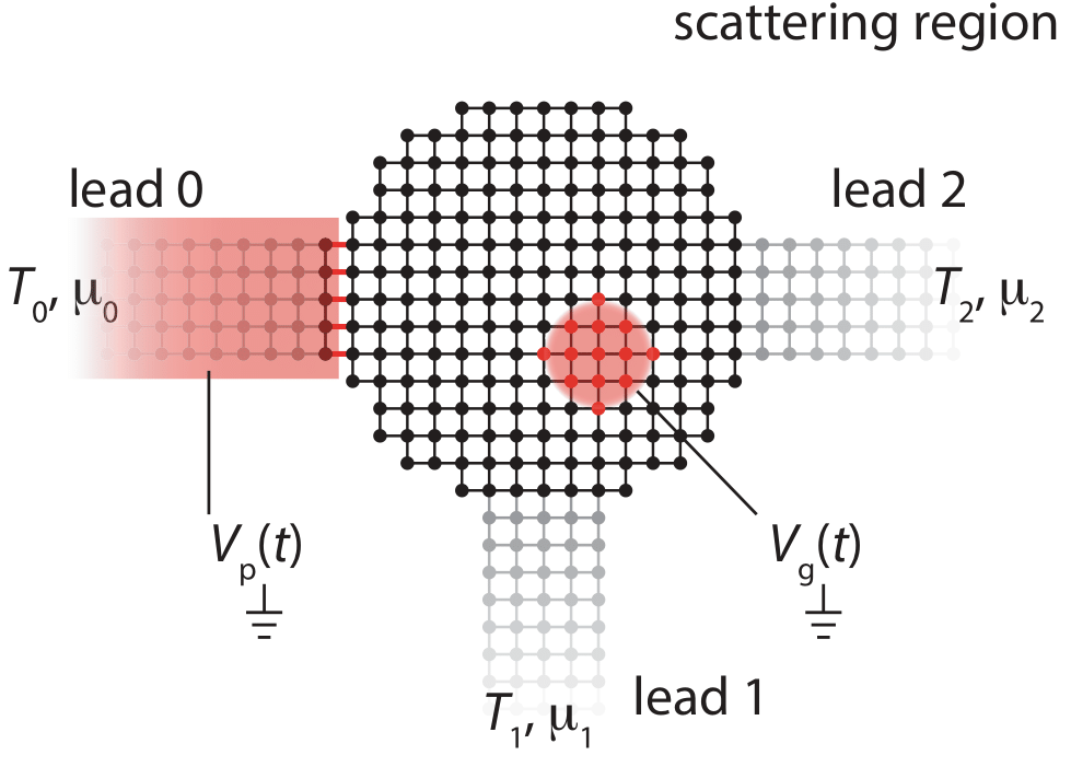
Sketch of a typical open quantum system which can be simulated with Tkwant. A central scattering region (in black) is connected to several leads (in grey). Each lead represents a translationally invariant, semi-infinite system in thermal equilibrium. Sites and hopping matrix elements are represented by dots and lines. The regions in red indicate a time-dependent perturbation, in this example a global voltage pulse \(V_p (t)\) on lead 0 and a time-dependent voltage \(V_g (t)\) on a gate inside the scattering region. The figure is taken from Ref. [1].
Input: A tight-binding Hamiltonian of generic form
as well as the chemical potential \(\mu\) and the temperature \(T\) in each lead.
Output: Time-dependent manybody expectation values, such as the electron density \(n_i(t) = \langle \hat{c}^\dagger_i \hat{c}_i \rangle\) an currents \(j_i(t) = i[\langle \hat{c}^\dagger_i \hat{c}_{i+1} \rangle - \langle \hat{c}^\dagger_{i+1} \hat{c}_{i} \rangle]\). We refer to Tkwant’s main paper Ref. [1] for the technical background.
2.1.1. Outline of the tutorial
The first tutorial sections Getting started: a simple example with a one-dimensional chain and Second example: Fabry-Perot interferometer dives directly into Tkwant with two simple examples. While the first one is a simple toy example for educative purpose, the second one is full fledged example, which has been described in detail in Ref. [1]. Tkwant’s core concepts to solve time-dependent manybody problems are explained in section Solving the many-body problem. Understanding this section allows one to use Tkwant effectively and to be able to perform realistic simulations. Another important tutorial section is Accounting for possible boundstates present in the system, as Tkwant does not handle boundstates automatically. Technical details are covered in the sections Advanced onebody settings, Advanced manybody settings and Boundary conditions. These sections can be skipped in a first tour and are intended for advanced users who are interested to change the default behavior. The two sections Parallelization with MPI and Logging introduce both topics at a beginner’s level and give some hands-on advice. Although not necessary for a basic understanding, these topics are likely to be relevant in practice. The section More examples section summarizes several complete Tkwant examples. Learning directly from the examples might be a good starting point especially for experienced Kwant users. Finally, we strongly recommend users to follow the advices in Frequent pitfalls encountered when doing Tkwant simulations to check their results for validity.
2.1.2. References
[1] T. Kloss, J. Weston, B. Gaury, B. Rossignol, C. Groth and X. Waintal, Tkwant: a software package for time-dependent quantum transport New J. Phys. 23, 023025 (2021), arXiv:2009.03132 [cond-mat.mes-hall].