2.8. Accounting for possible boundstates present in the system
Note
Quantum transport focuses on propagating states. However sometimes boundstates can play a major role (e.g. the Andreev states in Josephson junctions) or are simply there and must be taken into account. Tkwant does not handle boundstates automatically, but provides methods to detect and include them manually. The user must be careful, as neglecting existing boundstates can lead to incorrect results. While in the other tutorials boundstates were either not present or did not play a role, this tutorial demonstrates the detection and proper handling of boundstates in Tkwant with a simple example.
Boundstates are localized states inside the central region of an infinite scattering systems which decay exponentially in the leads. They are solutions of the Schrödinger equation and might occur in addition to the usual propagating states. General algorithms have been derived to calculate boundstates in arbitrary tight-binding system numerically [1], but they can often be calculated by simply diagonalizing a finite system that encompass the scattering region and a portion of the leads.
In this tutotiral, we illustrate the procedure to detect their presence, calculate them and include them in a Tkwant simulation on a simple toy example. We consider an infinite one-dimensional wire with a single impurity at a central site. For an attractive impurity potential, a single boundstate appears and its energy and its wavefunction can be calculated easily either numerically or analytically.
2.8.1. Model
We consider the simple tight-binding system of an infinite one-dimensional chain. At the center with lattice index zero there is an additional on-site potential with strength \(V\). In second quantization the Hamiltonian is
where \(c^\dagger_i\) (\(c_i\)) are the fermionic creation (annihilation) operator on site \(i\) and \(\gamma\) is the hopping matrix element. In the following we set \(\gamma = 1\) and work in dimensionless units.
2.8.2. Analytical calculation of the boundstate
To proceed, we consider the discrete Schrödinger equation
where \(H\) is the Hamiltonian matrix, \(\Psi = \{\psi_i, \psi_{i+1}, \ldots \}\) the projection of the wavefunction on the lattice sites \(i\) and \(E\) the energy. For our model the discrete Schrödinger equation can be written explicitly
with \(V_i = V \delta_{i, 0}\). The states are also required to be normalized and we fix the normalization to be:
One possible solution of Eqs. (3) and (4) are linar combination of plain-wave solution of the form \(\psi_n = c_1 e^{i k n} + c_2 e^{-i k n}\). These are the well-known scattering states with the corresponding dispersion relation \(E(k) = - 2 \gamma \cos(k)\). For the boundstates we are however looking for solutions of the form
with \(a, \lambda \in \mathcal{R}\) and \(\lambda > 0\). The normalization condition Eq. (4) requires that \(\lim_{i \rightarrow \pm \infty} \psi_i = 0\), such that \(|\lambda| < 1\). We can fix \(\lambda\) and the normalization constant \(a\) and \(\psi_0\) by simple wave function matching at the impurity. Equation (3) leads to
From Eq. (6c) and the ansatz Eq. (5) we find
For \(\lambda\) to be real the argument in the square root must be positive such that \(|E| \geq 2\). We will focus on solutions for attractive potentian \(V \leq 0\) with negative energy \(E\), such that only the root with the negative sign is possible as \(0 < \lambda < 1\). Together with Eqs. (6a, 6b) one finds the boundstate energies
such that the boundstate exists for all \(V < 0\). In terms of \(V\), Eq. (7) writes
The constant \(a\) can be fixed from the normalization condition Eq. (4):
Together with Eq. (6a) we find
2.8.3. Observables in presence of boundstates
The expectation value of an observable
can be calculated in in a wave-function based approach in the presence of boundstates as [2]
where \(\psi_{\alpha E}(t, i)\) is the scattering wave function for lead \(\alpha\), site index \(i\) and time \(t\), and \(f_\alpha\) is the Fermi function of lead \(\alpha\). The second term sums over the boundstate wavefunctions \(\psi_{b}\) with \(f(E_b)\) the Fermi function in the central region and \(E_b\) are the boundstate energies. Note that from a theoretical point of view, the Fermi function for the boundstate does not have to be at the same temperature or chemical potential than the leads. Hence it is not strictly speaking incorrect to ignore the bound states (i.e. assuming a large negative chemical potential for them) but often unphysical at least in the cases where the system is initially in thermal equilibrium. For the special case of the density we find
A very important remark for the detection of boundstates is that a given site contain exactly one electron when all the states are filled. Hence, if we diregard the Fermi functions in the above equation, one finds that Kwant [2] and Tkwant [3] give \(n(t, i) = 1\) in for all times \(t\) and all sites \(i\),
2.8.4. Numerical solution
We show in the following how to calculate the boundstates numerically for above model and how to include them into Tkwant. We first include standard Python packages alongside Kwant, Tkwant and KwantSpectrum [3].
import tkwant
import kwant
import kwantspectrum as ks

import numpy as np
import matplotlib.pyplot as plt
Characterization of the boundstate and comparison to the analytical result
We first implement two functions that return the analytical results: \(\texttt{bs_psi_func}\) calculate the boundstate wave function Eqs. (5, 9, 10) and \(\texttt{bs_energy_func}\) for the groundstate energy Eq. (8).
def bs_psi_func(v, i):
    lbda = 0.5 * (v + np.sqrt(v**2 + 4))
    lbda2 = lbda**2
    a = np.sqrt((1 - lbda2)/(1 + lbda2))
    return a * pow(lbda, abs(i))


def bs_energy_func(v):
    return - np.sqrt(v**2 + 4)
For the numerical solution we first implement the model Eq. (1) with Kwant. We also set the parameters such to have a boundstate present.
def make_system(L, V, a=1):

    lat = kwant.lattice.square(a=a, norbs=1)
    syst = kwant.Builder()

    # central system
    syst[(lat(i, 0) for i in range(-L, L))] = 0
    syst[lat(0, 0)] = V
    syst[lat.neighbors()] = -1

    # leads
    lead = kwant.Builder(kwant.TranslationalSymmetry((-a, 0)))
    lead[lat(0, 0)] = 0
    lead[lat.neighbors()] = -1
    syst.attach_lead(lead)
    syst.attach_lead(lead.reversed())

    return syst

# parameters
L = 20
V = -2.5

syst = make_system(L, V).finalized()

hamiltonian = syst.hamiltonian_submatrix()
In the previous lines, \(\texttt{hamiltonian}\) is the Hamiltonian matrix of the finite central system with size \((2 L + 1) \times (2 L + 1)\). This matrix could have been defined also directly, without using Kwant. One can plot the elements of this matrix for \(\{\psi_{-2}, \psi_{-1}, \psi_{0}, \psi_{1}, \psi_{2} \}\) to see that it corresponds indeed to Eq. (3):
np.array(np.real_if_close(hamiltonian[L-2:L+3, L-2:L+3]))
array([[ 0. , -1. ,  0. ,  0. ,  0. ],
       [-1. ,  0. , -1. ,  0. ,  0. ],
       [ 0. , -1. , -2.5, -1. ,  0. ],
       [ 0. ,  0. , -1. ,  0. , -1. ],
       [ 0. ,  0. ,  0. , -1. ,  0. ]])
Using standard linear algebra tools, we calculate the eigenvalues and eigenvectors of the matrix:
eigenvalues, eigenvectors = np.linalg.eigh(hamiltonian)
Boundstate energy
The eigenvalues correspond to discrete energy levels of the finite system. We plot the eigenvalues together with the energy dispersion of one lead, which corresponds to a semi-infinite system without any onsite energy.
spec = ks.spectrum(syst.leads[0])
momenta = np.linspace(-np.pi, np.pi, 500)

plt.plot([-1, 1], 2 * [eigenvalues[0]], c='#e15759', label=r'boundstate')

for i, energy in enumerate(eigenvalues[1:]):
    plt.plot([-1, 1], 2 * [energy], c='#f28e2b', label=r'plane waves' if i == 0 else "")

for band in range(spec.nbands):
    plt.plot(momenta, spec(momenta, band), label='contineous band')

plt.xlabel(r'$k$')
plt.ylabel(r'$E$')
plt.legend()
plt.show()
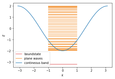
One finds that almost all eigenvalues are located inside the band opening. The corresponding states are plain-wave like solutions. The energy levels outsite the contineous band correspond to the boundstate. We find only one in this model. We copy the corresponding state and energy into
bs_energy = eigenvalues[0]
psi_bs = eigenvectors[:, 0]
and compare the energy to the analytical result:
bs_analyt = bs_energy_func(V)
print('boundstate energy (numeric): {:.4f}, (analytic): {:.4f}, diff: {:.4e}'.
      format(bs_energy, bs_analyt, np.abs(bs_energy - bs_analyt)))
boundstate energy (numeric): -3.2016, (analytic): -3.2016, diff: 1.7764e-15
Boundstate wave function
We can also plot the value of \(\psi_i\) on the lattice positions and compare to the analytical result. Summing up \(|\psi_i|^2\) on all sites we can also check that the normalization Eq. (4) holds:
sites = [s.pos[0] for s in syst.sites]
plt.plot(sites, np.real_if_close(psi_bs), label='numeric')
plt.plot(sites, [bs_psi_func(V, i) for i in sites], '--', label='analytic')

plt.xlabel(r'lattice site $i$')
plt.ylabel(r'$\psi_i$')
plt.legend()
plt.show()

print('normalization: {:.4f}'.format(np.sum(np.abs(psi_bs)**2)))

normalization: 1.0000
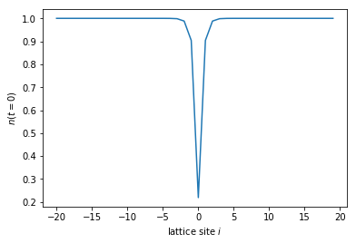
Wrong equilibrium density in Tkwant due to a missing boundstate
Although boundstates do not contribute to transport, a proper inclusion is nessessary when calculating manybody observables such as the density \(n(t, i)\). Here we show the error in the equilibrium density at initial time \(t=0\) when the existing boundstate is not properly included. To do this, we calculate the onside density using Eq. (13), neglecting the second term with the contribution of the boundstates. The numerical calculation is easily to perform with Tkwant, and we fill up all bands by setting the chemical potential \(\mu\) to a value higher than the largest band energy, which in this case is two. The deviation of the density from one near the impurity is the signature of the missing boundstate.
occupations = tkwant.manybody.lead_occupation(chemical_potential=4)
density_operator = kwant.operator.Density(syst)

state = tkwant.manybody.State(syst, tmax=1, occupations=occupations)
density = state.evaluate(density_operator)

plt.plot(sites, density)
plt.xlabel(r'lattice site $i$')
plt.ylabel(r'$n(t=0)$')
plt.show()
Detecting boundstates with Tkwant
Tkwant provides the boolian function \(\texttt{boundstates_present()}\) to check if boundstates are present:
syst_1 = make_system(L, V).finalized()
print("boundstates present: {}".format(tkwant.manybody.boundstates_present(syst_1)))

syst_2 = make_system(L, V=0).finalized()
print("boundstates present: {}".format(tkwant.manybody.boundstates_present(syst_2)))
boundstates present: True
boundstates present: False
Internally the function \(\texttt{boundstates_present()}\) checks for the density deviation from one as shown before.
Including boundstates in Tkwant
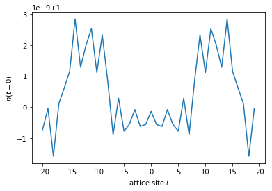
Tkwant does not automatically include boundstates. It merly provides a mechanism to manually add boundstates manually to the manybody state. To do this, the class \(\texttt{tkwant.manybody.State()}\) provides a method called \(\texttt{add_boundstate()}\). The boundstates must be added at initial time:
occupations = tkwant.manybody.lead_occupation(chemical_potential=4)
density_operator = kwant.operator.Density(syst)

state = tkwant.manybody.State(syst, tmax=1, occupations=occupations)
state.add_boundstate(psi_bs, bs_energy)
In case of several contributing boundstates they must be added one by one.
Note that the manybody wavefunction behaves normally, such that \(\texttt{evolve()}\) and \(\texttt{refine_intervals()}\) work as before and the boundstates evolved forward in time like the scattering states of the system. One can check that the density after the procedure is again one everywhere:
density = state.evaluate(density_operator)
plt.plot(sites, density)
plt.xlabel(r'lattice site $i$')
plt.ylabel(r'$n(t=0)$')
plt.show()
2.8.5. References
[1] M. Istas, C. Groth, A. R. Akhmerov, M. Wimmer, and X. Waintal, A general algorithm for computing bound states in infinite tight-binding systems SciPost Phys. 4, 26 (2018).
[2] C. W. Groth, M. Wimmer, A. R. Akhmerov, and X. Waintal, Kwant: a software package for quantum transport New J. Phys. 16, 063065 (2014).
[3] T. Kloss, J. Weston, B. Gaury, B. Rossignol, C. Groth and X. Waintal, Tkwant: a software package for time-dependent quantum transport New J. Phys. 23, 023025 (2021).