2.4. Time-dependent potentials and pulses
Tkwant uses Kwant to define the Hamiltonian of the tight-binding system. We show in the following how time-dependent onsite and coupling elements are defined. The latter can be used to simulate the injection of voltage pulses through the lead electrodes.
2.4.1. Time dependent onsite elements
Time-dependent gate potentials, aka \(V_g(t)\) in Getting started: a simple example with a one-dimensional chain,
act directly on the onsite elements of the Hamiltonian.
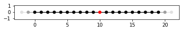
As an example, we define an infinitly long one-dimensional chain.
The central scattering region has 20 lattice sites (in black) and leads on both sides (in grey)
extend the system to \(\pm\) infinity.
On lattice site 10 (depicted in red), an additional time-dependent
\(\sin(\omega t)\) term is added to the onsite element. This can be done by defining
an appropriate onesite function, named onsite() in the example below:
import kwant
from math import sin

lat = kwant.lattice.square(a=1, norbs=1)
syst = kwant.Builder()

syst[(lat(x, 0) for x in range(20))] = 1
syst[lat.neighbors()] = -1

def onsite(site, fac, omega, time):
    return 1 + fac * sin(omega * time)

# add the time-dependent onsite potential
syst[lat(10, 0)] = onsite

lead = kwant.Builder(kwant.TranslationalSymmetry((-1, 0)))
lead[lat(0, 0)] = 1
lead[lat.neighbors()] = -1
syst.attach_lead(lead)
syst.attach_lead(lead.reversed())

# plot the system
kwant.plot(syst, site_color=lambda s: 'r' if s in [lat(10, 0)] else 'k',
           lead_color='grey');

syst = syst.finalized()
Kwant requires that the first element of
the onsite() function with name site is a
kwant.builder.Site
instance, while the other arguments are optional.
When initializing the solver tkwant.manybody.State the optional parameters
must be set by the params dictionary. Whereas the names for these optional parameters
are arbitrary, the name time is particular and will be interpreted
by Tkwant as the actual time variable.
import tkwant
state = tkwant.manybody.State(syst, tmax=100, params={'fac':0.1, 'omega':0.5})
The position of the time variable within the optional parameters in
the onsite() function is arbitrary.
See also
An example script which a time-dependent onsite potential is
1d_wire_onsite.py.
An example using optional parameters can be found in
fabry_perot.py.
2.4.2. Time dependent coupling elements
Time-dependent coupling elements of the Hamiltonian can be defined quite similar.
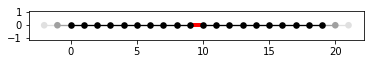
Again, we use an infinitly long one-dimensional chain with a central
scattering region of 20 lattice sites (in black) as an example. The coupling element between
matrix element 9 and 10 (highlighted in red) has an additional time-dependent
\(\sin(\omega t)\) term. This can be done by defining
a coupling function, named coupling() in the example below:
import kwant
from math import sin

lat = kwant.lattice.square(a=1, norbs=1)
syst = kwant.Builder()

syst[(lat(x, 0) for x in range(20))] = 1
syst[lat.neighbors()] = -1

def coupling(site1, site2, fac, omega, time):
    return -1 + fac * sin(omega * time)

# add the time-dependent coupling element
time_dependent_hopping = (lat(9, 0), lat(10, 0))
syst[time_dependent_hopping] = coupling

lead = kwant.Builder(kwant.TranslationalSymmetry((-1, 0)))
lead[lat(0, 0)] = 1
lead[lat.neighbors()] = -1
syst.attach_lead(lead)
syst.attach_lead(lead.reversed())

# plot the system
kwant.plot(syst, site_color='k', lead_color='grey',
           hop_lw=lambda a, b: 0.3 if (a, b) in [time_dependent_hopping] else 0.1,
           hop_color=lambda a, b: 'red' if (a, b) in [time_dependent_hopping] else 'k');

syst = syst.finalized()
Kwant requires that the first two elements of
the coupling() function to be instances of
kwant.builder.Site .
The rest is similar to above example with the time-dependent onsite elements.
import tkwant
state = tkwant.manybody.State(syst, tmax=100, params={'fac':0.1, 'omega':0.5})
2.4.3. Voltage pulses through a lead
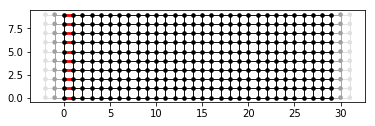
While the lead Hamiltonian does not depend explicitly on time, voltage pulses through a lead can be simulated by time-dependent coupling elements between the lead and system. In the current example, a time dependent potential drop is injected at a position \(i_b\), such that the system Hamiltonian becomes
\(\theta(x)\) is the Heaviside function and \(w(t)\) an arbitrary function parametrizing the time-dependent perturbation is applied to the system. One can absorb the effect of the time-dependent perturbation by a gauge transform. Defining the integrated pulse
this amount to simply replace the couplings \(\gamma\) from sites at \(i_b\) to site at \(i_b + 1\) by the time dependent couplings \(\gamma(t)\):
respectively the hermitian conjugate for the couplings from site \(i_b + 1\) to sites \(i_b\).
The Hamiltonian becomes
In this example we choose a Gaussian function
where \(v_p\) is some strenght and \(\tau\) accounts for the width of the pulse. Note the convention that the time-dependent perturbation has to start after time \(t=0\) and we have introduced a shift \(t_0\) in order to switch it on adiabatically. One finds
In the Python code we define directly the function \(\phi(t)\) and replace the coupling $gamma$ from sites 0 to 1 by the time dependent coupling $gamma(t)$ defined above. Note that the hermitian conjugate coupling from sites 1 to sites 0 is added by Kwant automatically.
import kwant
import cmath
from scipy.special import erf

def make_system(a=1, gamma=1.0, W=10, L=30):

    lat = kwant.lattice.square(a=a, norbs=1)
    syst = kwant.Builder()

    def phi(time):
        t0 = 100
        A = 0.00157
        tau = 24
        return A * (1 + erf((time - t0) / tau))

    # time dependent coupling with gaussian pulse
    def gamma_t(site1, site2, time):
        return - gamma * cmath.exp(- 1j * phi(time))

    #### Define the scattering region. ####
    syst[(lat(x, y) for x in range(L) for y in range(W))] = 4 * gamma
    syst[lat.neighbors()] = -gamma
    # time dependent lead-sys couplings from sites (x=0, y) to (x=1, y)
    time_dependent_hoppings = [(lat(1, y), lat(0, y)) for y in range(W)]
    syst[time_dependent_hoppings] = gamma_t

    #### Define and attach the leads. ####
    # Construct the left lead.
    lead = kwant.Builder(kwant.TranslationalSymmetry((-a, 0)))
    lead[(lat(0, j) for j in range(W))] = 4 * gamma
    lead[lat.neighbors()] = -gamma

    # Attach the left lead and its reversed copy.
    syst.attach_lead(lead)
    syst.attach_lead(lead.reversed())

    return syst, time_dependent_hoppings

syst, time_dependent_hoppings = make_system()

kwant.plot(syst, site_color='k', lead_color='grey',
           hop_lw=lambda a, b: 0.3 if (a, b) in time_dependent_hoppings else 0.1,
           hop_color=lambda a, b: 'red' if (a, b) in time_dependent_hoppings else 'k');
The special case of a time dependent coupling between the sites at the system-lead interface shown above can be written in more compact form. We first defines a system as before, but without the time dependent part.
import kwant

def make_system(a=1, gamma=1.0, W=10, L=30):

    lat = kwant.lattice.square(a=a, norbs=1)
    syst = kwant.Builder()

    #### Define the scattering region. ####
    syst[(lat(x, y) for x in range(L) for y in range(W))] = 4 * gamma
    syst[lat.neighbors()] = -gamma

    #### Define and attach the leads. ####
    # Construct the left lead.
    lead = kwant.Builder(kwant.TranslationalSymmetry((-a, 0)))
    lead[(lat(0, j) for j in range(W))] = 4 * gamma
    lead[lat.neighbors()] = -gamma

    # Attach the left lead and its reversed copy.
    syst.attach_lead(lead)
    syst.attach_lead(lead.reversed())

    return syst
The time dependent couplings are added by
import tkwant
from scipy.special import erf

def phi(time):
    t0 = 100
    A = 0.00157
    tau = 24
    return A * (1 + erf((time - t0) / tau))

syst = make_system()
added_sites = tkwant.leads.add_voltage(syst, 0, phi)
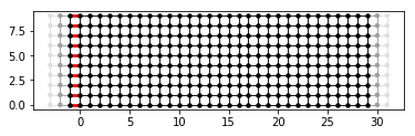
In fact, the routine adds new sites at the system-lead interface and
modifies syst. Note that syst must not be finalized. We can also
skip added_sites and call tkwant.leads.add_voltage without
return argument, if we are not interested in the added sites. The second
function argument of tkwant.leads.add_voltage corresponds to the
lead number, here 0, where the pulse is injected. We can show the
new sites with time-dependent couplings (in red) if we plot the system.
interface_hoppings = [(a, b)
                      for b in added_sites
                      for a in syst.neighbors(b) if a not in added_sites]
kwant.plot(syst, site_color='k', lead_color='grey',
           hop_lw=lambda a, b: 0.3 if (a, b) in interface_hoppings else 0.1,
           hop_color=lambda a, b: 'red' if (a, b) in interface_hoppings else 'k');
Note that in fact the system is not exactly the same as before due to
the additional sites (at x position -1), that were added. We could have constructed the
system with syst = make_system(L=29) to recover exactly the same
length as in the example before.
See also
An example script where a voltage pulses is injected through a lead is
fabry_perot.py.