2.5. Solving one-body problems
Tkwant can be used to simulate onebody and manybody dynamics. While the first tutorial examples covered manybody problems, this tutorial shows how to solve the onebody time-dependent Schrödinger equation. The examples in this section are taken from Ref. [1].
We like to solve the one-dimensional time-dependent Schrödinger equation
Starting from an initial condition of the generic form
we are interested in time evolution of the probability density
For this, the equation is discretized in space with \(x_i = a i\), where a is the grid spacing. The second derivative is approximated with a three-point finite difference scheme \(\partial_x^2 \psi(t, x) \approx (\psi(t, x_{i+1}) + \psi(t, x_{i-1}) - 2 \psi(t, x_{i}))/a^2\) The discretized equation has a simple matrix form
where
and we set the prefactor \(\hbar / (2 m a^2) = 1\) convenience.
2.5.1. Finite systems
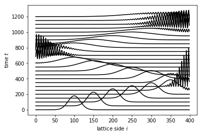
As a first example, above Schrödinger equation is solved for a finite system consisting of a finite number of scattering centers on a one-dimensional chain. A Gaussian wave package with a group velocity of \(v(k) = 1\) to the right is taken as initial condition. A sketch of the system is:

The actual parameters are: \(N = 400\) grid sites and the initial condition is taken as \(\psi(t = 0, j) = e^{- b (j - j_0)^2 + i k j}\) and the parameters are set to \(b = 0.001, j_0 = 100, k = \pi / 6\).
Defining the Hamiltonian matrix directly
One can directly define the Hamiltonian matrix in it’s tridiagonal form. The entire Tkwant code is
from tkwant import onebody
import numpy as np
import scipy
import matplotlib.pyplot as plt

# lattice sites and time steps
xi = np.arange(400)
times = np.arange(0, 1201, 50)

# initial condition
k = np.pi / 6
psi0 = np.exp(- 0.001 * (xi - 100)**2 + 1j * k * xi)

# hamiltonian matrix
diag = 2 * np.ones(len(xi))
offdiag = - np.ones(len(xi) - 1)
H0 = scipy.sparse.diags([diag, offdiag, offdiag], [0, 1, -1], dtype=complex)

# initialize the solver
wave_func = onebody.WaveFunction(H0, W=None, psi_init=psi0)

# loop over timesteps and plot the result
for time in times:
    wave_func.evolve(time)
    psi = wave_func.psi()
    density = np.real(psi * psi.conjugate())
    plt.plot(xi, 180 * density + time, color='black')

plt.xlabel(r'lattice side $i$')
plt.ylabel(r'time $t$')
plt.show()

The multiplication of the density by a prefactor (180 in above example) is only for representation purpose in order to make the shifted pulse visible. Note that the pulse is reflected at the boundaries, as the system is finite.
Defining the system using Kwant
The identical system can be build also with the help of Kwant. In this case, which is very similar to the tutorial example in the First steps, the Hamiltonian is defined implicitly.
from tkwant import onebody
import kwant
import numpy as np
import matplotlib.pyplot as plt

def make_system(L):

    # system building
    lat = kwant.lattice.square(a=1, norbs=1)
    syst = kwant.Builder()

    # central scattering region
    syst[(lat(x, 0) for x in range(L))] = 1
    syst[lat.neighbors()] = -1

    return syst

# build the system using kwant
syst = make_system(400).finalized()

# lattice sites and time steps
xi = np.array([site.pos[0] for site in syst.sites])
times = np.arange(0, 1201, 50)

# define observables using kwant
density_operator = kwant.operator.Density(syst)

# initial condition
k = np.pi / 6
psi0 = np.exp(- 0.001 * (xi - 100)**2 + 1j * k * xi)

# initialize the solver
wave_func = onebody.WaveFunction.from_kwant(syst, psi0)

# loop over timesteps and plot the result
for time in times:
    wave_func.evolve(time)
    density = wave_func.evaluate(density_operator)
    plt.plot(xi, 180 * density + time, color='black')

plt.xlabel(r'lattice side $i$')
plt.ylabel(r'time $t$')
plt.show()
2.5.2. Infinite systems
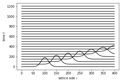
Now the Schrödinger equation is solved for an open system consisting of a infinite one-dimensional chain.

Again, a Gaussian wave package with a group velocity of \(v(k) = 1\) to the right is taken as initial condition.
Defining the system using Kwant
The same problem is now solved for an infinite system. The infinite system consists of a finite central region and two semi-infinite leads attached on both sides to extend the system to infinity. The central scattering region has again a size of \(N = 400\) grid sites. There is no boundary as before, such that the pulse is not reflected when it reaches the right edge.
from tkwant import onebody, leads
import kwant
import numpy as np
import matplotlib.pyplot as plt

def make_system(L):

    # system building
    lat = kwant.lattice.square(a=1, norbs=1)
    syst = kwant.Builder()

    # central scattering region
    syst[(lat(x, 0) for x in range(L))] = 1
    syst[lat.neighbors()] = -1

    # add leads
    sym = kwant.TranslationalSymmetry((-1, 0))
    lead_left = kwant.Builder(sym)
    lead_left[lat(0, 0)] = 1
    lead_left[lat.neighbors()] = -1
    syst.attach_lead(lead_left)
    syst.attach_lead(lead_left.reversed())

    return syst

# build the system using kwant
syst = make_system(400).finalized()

# lattice sites and time steps
xi = np.array([site.pos[0] for site in syst.sites])
times = np.arange(0, 1201, 50)

# define observables using kwant
density_operator = kwant.operator.Density(syst)

# initial condition
k = np.pi / 6
psi0 = np.exp(- 0.001 * (xi - 100)**2 + 1j * k * xi)

# make boundary conditions for the system with leads
boundaries = leads.automatic_boundary(syst.leads, tmax=max(times))

# initialize the solver
wave_func = onebody.WaveFunction.from_kwant(syst, psi0, boundaries)

# loop over timesteps and plot the result
for time in times:
    wave_func.evolve(time)
    density = wave_func.evaluate(density_operator)
    plt.plot(xi, 180 * density + time, color='black')

plt.xlabel(r'lattice side $i$')
plt.ylabel(r'time $t$')
plt.show()
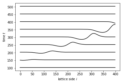
Infinite systems with initial scattering states
An infinite system which takes a scattering state as the initial condition has a special role in Tkwant as such a state form the basis for the manybody problem. Onebody scattering states are solution of the stationary Schrödinger equation
For the one-dimensional chain, the scattering states have the form
The scattering states are stationary solutions and therefore have no time evolution except the trivial phase oscillation. To obtain a non-trivial dynamics we perturb the system by an explicit time-dependent Hamiltonian matrix of the form
Here, \(H_{0, ij}\) is the time-independent part, which we take similar as before, \(\theta(x)\) is the Heaviside function and \(w(t)\) is a function that parametrizes the time-dependent perturbation. We choose
and apply a similar gauge transform as in Time-dependent potentials and pulses.
In the first example we calculate the initial scattering state
explicitly using Kwant. In scattering_states(0)[0] below, the first zero in round brackets corresponds to the lead index
whereas the second zero in square brackets corresponds to the mode index. The entire code is
from tkwant import onebody, leads
import kwant
import numpy as np
from scipy.special import erf
import matplotlib.pyplot as plt

def make_system(L):

    # system building
    lat = kwant.lattice.square(a=1, norbs=1)
    syst = kwant.Builder()

    # central scattering region
    syst[(lat(x, 0) for x in range(L))] = 1
    syst[lat.neighbors()] = -1

    # add leads
    sym = kwant.TranslationalSymmetry((-1, 0))
    lead_left = kwant.Builder(sym)
    lead_left[lat(0, 0)] = 1
    lead_left[lat.neighbors()] = -1
    syst.attach_lead(lead_left)
    syst.attach_lead(lead_left.reversed())

    return syst

# build the system using kwant
syst = make_system(400)

# add the voltage pulse
def gaussian(time):
    return 1.57 * (1 + erf((time - 40) / 20))

leads.add_voltage(syst, 0, gaussian)
syst = syst.finalized()

# lattice sites and time steps
xi = np.array([site.pos[0] for site in syst.sites])
times = np.arange(0, 401, 50)

# define observables using kwant
density_operator = kwant.operator.Density(syst)

# make boundary conditions for the system with leads
boundaries = leads.automatic_boundary(syst.leads, tmax=max(times))

# initialize the solver
# create a time-dependent wavefunction that starts in a scattering state
# originating from the left lead as initial state
scattering_states = kwant.wave_function(syst, energy=0., params={'time': 0})
lead = 0
mode = 0
psi_st = scattering_states(lead)[mode]

# initialize the solver starting in the scattering state
wave_func = onebody.WaveFunction.from_kwant(syst, psi_st, boundaries=boundaries,
                                            energy=0.)

# loop over timesteps and plot the result
for time in times:
    wave_func.evolve(time)
    density = wave_func.evaluate(density_operator)
    plt.plot(xi, 180 * density + time, color='black')

plt.xlabel(r'lattice side $i$')
plt.ylabel(r'time $t$')
plt.show()

There is a simpler way in Tkwant to set up the initial scattering states
using onebody.ScatteringStates.
The code below if fully equivalent to the above example:
from tkwant import onebody, leads
import kwant
import numpy as np
from scipy.special import erf
import matplotlib.pyplot as plt

def make_system(L):

    # system building
    lat = kwant.lattice.square(a=1, norbs=1)
    syst = kwant.Builder()

    # central scattering region
    syst[(lat(x, 0) for x in range(L))] = 1
    syst[lat.neighbors()] = -1

    # add leads
    sym = kwant.TranslationalSymmetry((-1, 0))
    lead_left = kwant.Builder(sym)
    lead_left[lat(0, 0)] = 1
    lead_left[lat.neighbors()] = -1
    syst.attach_lead(lead_left)
    syst.attach_lead(lead_left.reversed())

    return syst

# build the system using kwant
syst = make_system(400)

# add the voltage pulse
def gaussian(time):
    return 1.57 * (1 + erf((time - 40) / 20))

leads.add_voltage(syst, 0, gaussian)
syst = syst.finalized()

# lattice sites and time steps
xi = np.array([site.pos[0] for site in syst.sites])
times = np.arange(0, 401, 50)

# define observables using kwant
density_operator = kwant.operator.Density(syst)

# initialize the solver
wave_func = onebody.ScatteringStates(syst, energy=0., lead=0,
                                     tmax=max(times))[0]

# loop over timesteps and plot the result
for time in times:
    wave_func.evolve(time)
    density = wave_func.evaluate(density_operator)
    plt.plot(xi, 180 * density + time, color='black')

plt.xlabel(r'lattice side $i$')
plt.ylabel(r'time $t$')
plt.show()
See also
Advanced settings to solve the onebody Schrödinger equation are described in section Advanced onebody settings. Further examples are given in section More examples.
2.5.3. References
[1] T. Kloss, J. Weston, B. Gaury, B. Rossignol, C. Groth and X. Waintal, Tkwant: a software package for time-dependent quantum transport New J. Phys. 23, 023025 (2021).