2.9. Self-consistent Tkwant: a generic solver for time-dependent mean field calculations

In its usual mode, Tkwant deals with non-interacting particles where the system Hamiltonian is quadratic in the fermion operators. While many problems can be studied at this level, there are also many situations where one wants to take interactions into account, at least at some approximate level. One simple example are plasmonic excitations in Luttinger liquids, where the bare Fermi velocity is renormalized to higher values due to the electron-electron interaction [1]. One can describe such a system by a one dimensional Hubbard like Hamiltonian of the form

\[\begin{equation} H = \sum_{<ij>,\sigma} \gamma_{ij} c^\dagger_{i\sigma} c_{j\sigma} + U \theta(t) \sum_i c^\dagger_{i\uparrow}c_{i\uparrow}c^\dagger_{i\downarrow} c_{i\downarrow} , \tag{1} \end{equation}\]

A common approximation strategy is to decouple the interaction term into a quadratic form such that one could solve it. At the time-dependent Hartree-Fock level our approximate Hamiltonian would read

\[\begin{equation} H^{\textrm{HF}} = \sum_{<ij>,\sigma} \gamma_{ij} c^\dagger_{i\sigma} c_{j\sigma} + U \sum_{i, \sigma} \langle c^\dagger_{i\sigma} c_{i\sigma}\rangle(t) c^\dagger_{i\bar \sigma} c_{i\bar \sigma}. \tag{2} \end{equation}\]

To solve the Schrödinger equation with above Hamiltonian numerically is however much more involved as for a non-interacting problem, as the time-dependent onsite density \(\langle c^\dagger_{i\sigma} c_{i\sigma}\rangle(t)\) enters into the Hamiltonian matrix and must be calculated self-consistently during the time evolution. This tutorial discusses a new Tkwant class that solve this class of self-consistency problems and more generally any problem where the Hamiltonian depends not only on time but also on some time-dependent observable(s).

After explaining the general concept of the solver class we will demonstrate its flexibility on three concrete examples taken from recent articles: A self-consistent Hartree approach for Luttinger liquids [1], a microscopic Bogoliubov-deGennes equation describing a superconducting Josephson junction [2], and the solution of the Landau-Lifshitz-Gilbert equations for an interacting spin system [3].

2.9.1. Problem definition

The self-consistent solver class discussed in this tutorial is designed for problems with a Hamiltonian matrix of generic form

\[\begin{equation} \mathbf{H} = \mathbf{H}_0 + \mathbf{W}(t) + \mathbf{Q}[t, y(t)] . \tag{3} \end{equation}\]

In above equation, the first two terms \(\mathbf{H}_0\) and \(\mathbf{W}\) are the usual static and time-dependent parts while \(\mathbf{Q}\) is a term to be evaluated self-consistently and \(y(t)\) is an observable. For the concrete example of the Hartree-Fock Hamiltonian in Eq. (2), the matrix elements of \(\mathbf{Q}\) would be

\[\begin{equation} \mathbf{Q}_{ij}(t) = U \delta_{ij} y_i(t), \qquad y(t) = \langle c^\dagger_{i} c_{i}\rangle(t) \tag{4} \end{equation}\]

while \(y(t)\) is the time-dependent onsite density (the spin is ignored for simplicity).

The concrete form of \(\mathbf{Q}\) is provided by the user. It depends on the specific physical system and the decoupling approximation used. Tkwant considers the case in which \(\mathbf{Q}\) is an arbitrary function - or even functional- of a manybody expectation value

\[\begin{equation} y (t) = \sum_{\alpha ij} \int \frac{dE}{2 \pi} f_\alpha(E) \psi_{\alpha E}^*(t,i) \mathbf{Y}_{ij} \psi_{\alpha E}(t,j).\tag{5} \end{equation}\]

In above equation, \(f_\alpha\) refers to is the Fermi function of lead \(\alpha\) and \(\hat{\mathbf{Y}}\) is an observable of the form

\[\begin{equation} \label{eq:observable} \hat{\mathbf{Y}} = \sum_{i,j} \mathbf{Y}_{ij} \hat{c}^\dagger_i \hat{c}_j \tag{6} \end{equation}\]

and \(\psi_{\alpha E}(t, i)\) is the scattering wave function for lead \(\alpha\), site index \(i\), time \(t\) and energy \(E\). Each scattering wave function evolves according to the time-dependent Schrödinger equation

\[\begin{equation} i \partial_t \psi_{\alpha E}(t, i) = \sum_j\mathbf{H}_{ij}[t, \Psi] \psi_{\alpha E}(t,j) . \tag{7} \end{equation}\]

Due to the coupling of the scattering modes via \(\mathbf{Q}\) and \(y\), the Hamiltonian in Eq. (3) becomes implicitely a functional of the manybody wavefunction \(\Psi\), (i.e. of the ensemble of all onebody wavefuction \(\psi_{\alpha E}\)). The calculations of the observable \(y(t)\) uses the same functions as for other observables of interest (see Ref. [4]). \(y(t)\) may or may not be the actual observable that one actually wants to compute. This formulation of the problem is sufficiently general to encompass many different situations. The table below illustrates the physical meaning of \(y\) and \(\mathbf{Q}\) for the three different examples [1-3]. The first problem corresponds to the self-consistent time-dependent Hartree approximation where at each time step, one would solve the Poisson equation to update the potential seen by the electrons. In the second a Josephson junctions injects a time-dependent current (\(y(t)\)) into a classical LRC circuit which in turns affects the electrical potential seen by the junction (\(\mathbf{Q}\)). In the third, the spin current (\(y(t)\)) creates a torque that affects the classical magnetization whose classical dynamics is described by a Landau Lifshitz Gilbert (LLG) equation which in turns affects the dynamics of the electrons (\(\mathbf{Q}\)). Many multi-physics problems can be described in this way.

problem	observable \(y(t)\)	mean-field potential \(\mathbf{Q}[t, y(t)]\)
ee interaction	density	electrostatic potential (Poisson equation)
Josephson junction	current	bias voltage (classical electric circuit equations)
spintronics	spin density	spin dependent potential (LLG equation)

To solve a self-consistent problem with Tkwant in practice, the user needs to implement two classes: One is the operator \(\hat{Y}\) for calculating \(y\) and the other one is for computing \(\mathbf{Q}\). In many situations however, as for instance the first two examples [1, 2], \(y\) can be calculated with Kwant’s standard operators, such that only one single class for \(\mathbf{Q}\) needs to be implemented. A sketch of a time-evolution step with the self-consistent solver is given in the figure below, where the arrows indicate the flow of data between the different code blocks.

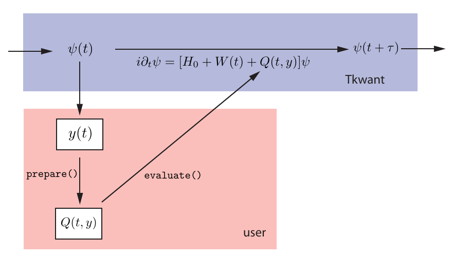
Figure 1: Sketch of a time-evolution step in a self-consistent Tkwant simulation. The self-consistent potential \(\mathbf{Q}\) must be implemented by the user (orange box) as a Python class which provides a prepare() and an evaluate() method, see API of the self-consistent solver and its helper classes.

To continue, we showcase the self-consistent Tkwant solver on a simple toy example.

2.9.2. Toy example for a self-consistent Tkwant simulation

Our toy example does not solve a problem of physical interest, it is for educational purpose only. We consider the tight-binding Hamiltonian

\[\begin{equation} H = - \sum_{i= \infty}^\infty (c^\dagger_{i+1} c_{i} + \text{h.c.}) + V(t) c^\dagger_{0} c_{0} - [J e^{-i \langle c^\dagger_1 c_1 \rangle(t)} - 1] c^\dagger_{2} c_{1} + \text{h.c.} \tag{8} \end{equation}\]

where \(c^\dagger_{i}\) (\(c_{i}\)) is the fermionic creation (annihilation) operator on site \(i\) and \(V(t)= \tanh(t)\) is an external potential acting only on site 0. The interaction with strength \(J\) is described by the third term and modulates the hopping amplitude between sites 1 and 2. In this example, the expectation value \(y(t)\) corresponds to the electron density on site 1:

\[\begin{align} y(t) \equiv \langle c^\dagger_1 c_1 \rangle(t) = \sum_\alpha \int \frac{dE}{2\pi} f_0(E) |\psi_{\alpha E}(1,t)|^2 .\tag{9} \end{align}\]

From above Hamiltonian Eq. (8) one reads of the non-interacting static part \([\mathbf{H}_0]_{ij} = - (\delta_{i, j + 1} + \delta_{i, j - 1})\) as well as the time-dependent part \(\mathbf{W}_{00}(t) = V(t)\) of the Hamiltonian matrix. The matrix \(\mathbf{Q}\) of the interaction contribution is a simple function of \(y(t)\) and has two nonzero elements:

\[\begin{align} \mathbf{Q}_{21}(y(t)) = - [e^{-i y(t)} - 1], \quad \mathbf{Q}_{12}(y(t)) = \mathbf{Q}_{21}^*(y(t)).\tag{10} \end{align}\]

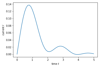
We consider each lead to be at zero temperature, the Fermi energy to be at \(E_F = -1.5\) (the bottom of the band is at an energy of \(-2\)) and the coupling to be \(J = 0.1\). Finally, the observable which we would like to measure is the current flowing from site 2 to site 3. It is defined as:

\[\begin{equation} I(t) = - 2 i \textrm{Im} \sum_\alpha \int \frac{d E}{2 \pi} f_\alpha(E) \psi_{\alpha E}^*(t, 3) H_{3,2} \psi_{\alpha E}(t, 2). \tag{11} \end{equation}\]

Let us now show how to solve this problem numerically with Tkwant.

(I) Setting up the non-interacting wave-function \(\Psi_0\)

First, one needs a Tkwant wavefunction instance as tkwant.manybody.WaveFunction, which corresponds to the time-dependent manybody wavefunction \(\Psi\). Note that one cannot use the high-level routine tkwant.manybody.State() as the automatic integral refinement of this class is not compatible with the self-consistency algorithm. How to use the low-level many-body wavefunction with tkwant.manybody.WaveFunction() is described in the tutorial: manybody low-level manual approach.

import tkwant
import kwant
import kwantspectrum

import functools
import numpy as np
import math
import scipy
import matplotlib.pyplot as plt


def vt(site, time):
    return math.tanh(time)

def make_system(L=4):

    lat = kwant.lattice.square(a=1, norbs=1)
    syst = kwant.Builder()

    #-- central scattering region
    # H_0
    syst[(lat(x, 0) for x in range(L))] = 0
    syst[lat.neighbors()] = -1

    # W(t)
    syst[lat(0, 0)] = vt

    #-- leads
    sym = kwant.TranslationalSymmetry((-1, 0))
    lead_left = kwant.Builder(sym)
    lead_left[lat(0, 0)] = 0
    lead_left[lat.neighbors()] = -1
    syst.attach_lead(lead_left)
    syst.attach_lead(lead_left.reversed())

    return syst, lat

syst, lat = make_system()
syst = syst.finalized()

times = np.linspace(0, 5, 51)

# calculate the spectrum E(k) for all leads
spectra = kwantspectrum.spectra(syst.leads)

# Lead occupation
occupations = tkwant.manybody.lead_occupation(chemical_potential=-1.5, temperature=0)

# define boundary conditions
bdr = tkwant.leads.automatic_boundary(spectra, tmax=max(times))

# calculate the k intervals for the quadrature
interval_type = functools.partial(tkwant.manybody.Interval, order=5,
                                  quadrature='gausslegendre')
intervals = tkwant.manybody.calc_intervals(spectra, occupations, interval_type)
intervals = tkwant.manybody.split_intervals(intervals, number_subintervals=1)

# calculate all onebody scattering states at t = 0
tasks = tkwant.manybody.calc_tasks(intervals, spectra, occupations)
psi_init = tkwant.manybody.calc_initial_state(syst, tasks, bdr)

# set up the manybody wave function
wave_function = tkwant.manybody.WaveFunction(psi_init, tasks)

(II) Implementing the class to calculate \(y(t)\)

In our example \(y(t)\) is the density on site 1 as defined in Eq. (9). We therefore do not need to implement a class but can use the standard Kwant operator to calculate the onsite density:

y_operator = kwant.operator.Density(syst, where=[lat(1, 0)])

(III) Implementing the class to calculate the mean-field potential \(\mathbf{Q}[t, y]\)

The class to calculate the \(\mathbf{Q}\) matrix must provide two methods: The first method prepare() is a precompute step. In our case this method only receives and stores the function \(y(t)\). The second method evaluate() actually calculates \(\mathbf{Q}\). We implement directly Eq. (10) and return \(\mathbf{Q}\) in form of a sparse matrix.

class MeanFieldPotentialQ:
    def __init__(self, coupling_j, size):
        self._coupling_j = coupling_j
        self._size = size

    def prepare(self, yt, tmax):
        """Pre-calculate the interaction contribution Q(t)"""
        self._yt = yt

    def evaluate(self, time):
        """Return the interaction contribution Q(t) evaluated at time *t*"""
        q21 = 1 - np.exp( - 1j * self._yt(time)) * self._coupling_j
        row = [2, 1]
        col = [1, 2]
        data = [q21, q21.conjugate()]
        return scipy.sparse.coo_matrix((data, (row, col)), dtype=complex,
                                       shape=(self._size, self._size))

q_potential = MeanFieldPotentialQ(coupling_j=0.1, size=len(syst.sites))

(IV) Setting up the self-consistent solver

Tkwant provides the class SelfConsistentState() to solve self-consistent mean-field problems. We can instatiate it directly from the three objects which represent \(\Psi_0\), \(\hat{Y}\) (which allows to calculate \(y\)) and \(\mathbf{Q}\):

sc_wavefunc = tkwant.interaction.SelfConsistentState(wave_function, y_operator, q_potential)

Apart from that, sc_wavefunc behaves like a standard Tkwant wavefunction, such that it has an evolve() and an evaluate() method, to be evolved in time and to compute the expectation value of an operator.

current_operator = kwant.operator.Current(syst, where=[(lat(3, 0), lat(2, 0))])

currents = []
for time in times:
    sc_wavefunc.evolve(time)
    current = sc_wavefunc.evaluate(current_operator)
    currents.append(current)

plt.plot(times, currents)
plt.xlabel(r'time $t$')
plt.ylabel(r'current $I$')
plt.show()

2.9.3. API of the self-consistent solver and its helper classes

The following section explains in more details the API of the class SelfConsistentState(), as well as the two additional classes which represent the \(Y\) operator and mean-field potential \(\mathbf{Q}[t, y]\). These two classes must be implemented by the user and require a specific API.

The class to calculate \(y(t)\)

The class to represent the operator \(\hat{Y}\) must have a __call__ method with an API similar to a standard Kwant operator:

class MyOperatorY:

    def __call__(self, bra, ket=None, args=(), *, params=None):
        """Compute the expectation value ⟨ψ|Y|ψ⟩ with a onebody wave-function ψ,
           API similar to a Kwant operator"""
        .
        .  Compute <ψ|Y|ψ>, this step can be compute intensive.
        .
        return observable

The retured observable must be a one-dimensional numpy array. The self-consistent solver class tkwant.interaction.SelfConsistentState() described below will call a MyOperatorY instance to calculate the expectation value \(y(t)\) in Eq. (5). The class MyOperatorY can be compute intensive, as it is called only after a (large) timestep \(\tau\), as explained later on.

The class to calculate the mean-field potential \(\mathbf{Q}[t, y]\)

The class to calculate the Hamiltonian matrix \(\mathbf{Q}[t, y]\) must provide two methods with the following API:

class MyMeanFieldPotentialQ():

    self._tmax = 0

    def prepare(self, yt, tmax):
        """Pre-calculate the interaction term Q[t, y] for time t in [tmin, tmax]"""
        self._tmin = self._tmax
        self._tmax = tmax
        .
        . Prepare Q(t) calculation, this step can be computationally intensive.
        .
        return

    def evaluate(self, time):
        """Return the Q[t, y] matrix evaluated at time *t*"""
        .
        . Calculate Q[t, y] matrix, this step should be fast.
        .
        return qt_matrix

At this stage, the reader might wonder why the class in charge of calculating \(\mathbf{Q}[t, y]\) requires one to implement two methods and not just a single one. The rationale for this as well as how to split the work between the two methods will be explained below in the section Behind the scene: Timescale decoupling. For the moment, one must only understand that these methods are needed for computational efficiency. prepare() will be called few times and must therefore do all the heavy work while evaluate() will be called often and must be very fast.

• \(\texttt{prepare()}\) has the signature (yt, tmax). Here yt is a function which can be called with a time \(t\) and which evaluates \(y(t)\) for \(t \leq t_{max}\). Once prepare() is called, the previous value of \(t_{max}\) [that was set in the previous call to prepare()] becomes the new \(t_{min}\) and \(t \geq t_{min}\). In a typical setting, prepare() calculates \(\mathbf{Q}[t, y(t)]\) for a few values of \(t\) in the interval \([t_{min}, t_{max}]\) and then constructs an interpolant of \(\mathbf{Q}[t, y(t)]\) for any value ot \(t\) in this range. The value of the interpolant will be returned by evaluate().

• \(\texttt{evaluate()}\) returns the interaction contribution \(\mathbf{Q}[t, y(t)]\) for a given time \(t\). The return type can be any matrix like object, which allows to perform a matrix-vector product with the wave function in the central scattering system. The time argument of evaluate() is always in between tmin and tmax, i.e. in between the value of tmax used in the second to last and last call to prepare().

Setting up the self-consistent solver

Tkwant provides the solver SelfConsistentState() for to solve time-dependent self-consistency equations. It is instatiated as:

sc_wavefunc = tkwant.interaction.SelfConsistentState(wavefunc,
                                                     y_operator,
                                                     q_potential)

In above line, wavefunc is an instance of tkwant.manybody.WaveFunction, y_operator an instance of MyOperatorY and q_potential an instance of MyMeanFieldPotentialQ. These three objects represent \(\Psi_0\), \(\hat{Y}\) and \(\mathbf{Q}[t, y]\). The sc_wavefunc object represents the wave function for the self-consistent state. This wave-function is defined similar to the non-interacting wave-function in Ref. [4], but the individual modes are solutions of the non-linear Schrödinger equation (7). Apart from that, sc_wavefunc behaves like a standard Tkwant wavefunction, such that it has an evolve() and an evaluate() method, to be evolved in time and to compute the expectation value of an operator.

2.9.4. Behind the scene: Timescale decoupling

Let’s now explain how Tkwant uses the routines prepare() and evaluate() to integrate the equations of motions. In a typical simulation, one needs a few hundred values of the energy to compute an observable, so that a self-consistent Tkwant calculation amounts to solving a set of hundreds of coupled (non-linear) Schrodinger equations in parallel. Such a calculation cannot be done by brute force on large systems. The approach taken in self-consistent Tkwant to address this problem efficiently is to leverage on the fact that observables typically evolve very slowly with respect to individual wave-functions. This seperation of scales is used by Tkwant to implement a two timesteps integrator.

More precisely, the individual wavefunctions \(\psi_{\alpha E}(t)\) vary typically on a timescale \(d t\) of the order of the inverse of band width or inverse of the Fermi energy. On the other hand, the observables and therefore the self-consistent potential \(\mathbf{Q}(t) \equiv \mathbf{Q}[t, y(t)]\) vary on a time scale \(\tau\). In many situations of interest \(\tau\gg dt\) which can be used to get an important speed up of the calculations. A sketch of the evolution of \(\mathbf{Q}(t)\) and of \(\psi_{\alpha}(t)\) is shown in the figure 2 below.

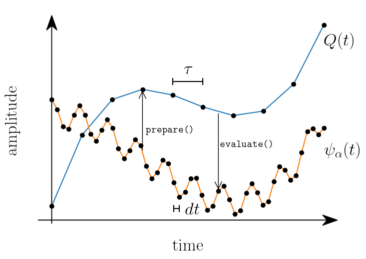
Figure 2: Sketch to illustrate the fast evolution of the wave function \(\psi_{\alpha}(t)\) (orange) on a timescale \(dt\) compared to the slower changing mean-field potential \(\mathbf{Q}(t)\) (blue) on a timescale \(\tau\). The dots represent the time points on which \(\psi_{\alpha}(t)\) and \(\mathbf{Q}(t)\) are evaluated to solve the Schrödinger equation numerically.

The doubly adaptive integrator of self-consistent Tkwant uses the following algorithm to integrate the problem from \(t\) to \(t + \tau\):

• First, we extrapolate \(y(t)\) from the interval \([t-\tau,t]\) to the interval \([t,t+\tau]\) using a linear extrapolation (default) or any user defined extrapolation scheme. The extrapolated value is noted \(\tilde{y}(t)\).

• Second, the routine prepare() is called with \(t_{max} =t +\tau\) and yt given by \(\tilde{y}(t)\). The role of prepare() is to precompute \(\mathbf{Q}[t, y]\) in the interval \([t,t+\tau]\) from the extrapolated value \(\tilde{y}(t)\). Typically, prepare() would compute \(\mathbf{Q}[t, y]\) for a few points in the interval, then compute an interpolant between these points to be returned by evaluate(). In the simplest scheme, one can just consider that \(\mathbf{Q}[t, y]\) is constant in the interval \([t,t+\tau]\) and use \(\tilde{y}(t + \tau/2)\) for its computation. One can also perform no interpolation of \(\mathbf{Q}[t, y]\) at all (as in the previous toy example). However in that case the computation might become extremely inefficient.

• Third, the different Schrödinger equations for the individual wave-functions \(\psi_{\alpha E}(t)\) are integrated from \(t\) to \(t + \tau\) using the usual adaptive Tkwant integrator with \(\mathbf{Q}[t, y]\) considered as a given external time-dependent Hamiltonian, as returned by the method evaluate(). These integrations are discretized on a very small time scale \(dt \ll \tau\), hence the method evaluate() will be called much more often (\(\sim\tau/dt\)) than prepare().

• Fourth, the value of the observable \(y(t+\tau)\) is computed. It is compared to the extrapolated value \(\tilde{y}(t)\). If these two quantities differ by more than a predefined tolerance, then \(\tau\) is reduced in order to control the extrapolation error.

2.9.5. Real-live examples of self-consistent Tkwant simulations:

We now demonstrate complete self-consistent simulation examples take from three recent publications. After introducing the relevant equations we will concentrate mainly on their form and the practical implementation to solve them and refer to the corresponding articles for the whole story.

1) Luttinger liquid physics from time-dependent Hartree approximation

The propagation of plasmonic excitations in quasi-one dimensional wires has been studied in Ref [1]. The initial Hamiltonian is

\[\begin{equation} H = \sum_{<ij>,\sigma} \gamma_{ij} c^\dagger_{i\sigma} c_{j\sigma} + \sum_{i\sigma} V_{\rm b}(t) \theta(i_{\rm b} -i) c^\dagger_{i\sigma} c_{i\sigma} + U \sum_i s(i) (c^\dagger_{i\uparrow}c_{i\uparrow} - n_0)(c^\dagger_{i\downarrow} c_{i\downarrow} - n_0) \tag{12} \end{equation}\]

where \(c^\dagger_{i\sigma}\) (\(c_{i\sigma}\)) is the fermionic creation (annihilation) operator on site \(i\) and spin \(\sigma = \{ \uparrow, \downarrow \}\), \(V_{\rm b}(t)\) is a time-dependent bias voltage, \(\theta(x)\) the Heaviside step-function and the hopping \(\gamma_{ij} = 1\) for nearest neighbour sites. Moreover \(U\) the interaction strength, \(n_0\) the equilibrium density and \(s(i)\) allows to parametrize the spacial extent of the interacting zone. For convenience, we set \(s(i) = 1\) and also focus on the one-dimensional case. After Hartree-Fock decoupling, the Hamiltonian matrix is

\[\begin{equation} \mathbf{H}_{ij} = \gamma_{ij} + V_{\rm b}(t) \theta(i_{\rm b} -i) + U s(i) (n(i,t)-n_0). \tag{13} \end{equation}\]

In terms of the splitting Eq. (3), the matrix elements of the first two matrices are \(H_0 = \gamma_{ij}\) and \(W(t) = (e^{- i \int_0^t dt' V_{\rm b}(t')} - 1) \delta_{i_{\rm b}, i_{\rm b}+1}\), where the bias potential \(V_{\rm b}(t)\) has been absorbed into a time-dependent coupling by a standard gauge transform. The third term is the self-consistent Hartree contribution

\[\begin{equation} \mathbf{Q}_{ij}(t) = U (n(i,t)-n_0) \delta_{ij}, \tag{14} \end{equation}\]

with \(n_0 = n(i, t=0)\). The local density is calculated from the wavefunction as

\[\begin{equation} n(i, t) = \sum_\alpha \int \frac{dE}{2\pi} f_0(E) |\psi_{\alpha E}(i,t)|^2 . \tag{15} \end{equation}\]

We now show the corresponding Tkwant implementation to compute the time evolution of the density \(n(i, t)\).

(I) Non-interacting wavefunction \(\Psi_0\)

We start with the non-interacting manybody wave function. Even though lenghly, this part is taken almost literally from the low-level approach, see manybody low-level manual approach. Note however that the interval order and the number of subinterval, aka order and number_subintervals, were lowered to speed up the simulation for the tutorial:

import tkwant
import kwant
import kwantspectrum

import functools
import numpy as np
import scipy
import matplotlib.pyplot as plt


def gaussian(time):
    t0 = 50
    A = 0.31415926535
    sigma = 12.01122
    return A * (1 + scipy.special.erf((time - t0) / sigma))


def make_system(L=100):

    # system building
    lat = kwant.lattice.square(a=1, norbs=1)
    syst = kwant.Builder()

    # central scattering region
    syst[(lat(x, 0) for x in range(L))] = 1
    syst[lat.neighbors()] = -1

    # add leads
    sym = kwant.TranslationalSymmetry((-1, 0))
    lead_left = kwant.Builder(sym)
    lead_left[lat(0, 0)] = 1
    lead_left[lat.neighbors()] = -1
    syst.attach_lead(lead_left)
    syst.attach_lead(lead_left.reversed())

    return syst, lat


syst, lat = make_system()
tkwant.leads.add_voltage(syst, 0, gaussian)
syst = syst.finalized()

sites = [site.pos[0] for site in syst.sites]
times = [20, 40, 60, 80]

density_operator = kwant.operator.Density(syst)

# calculate the spectrum E(k) for all leads
spectra = kwantspectrum.spectra(syst.leads)

# estimate the cutoff energy Ecut from T, \mu and f(E)
# All states are effectively empty above E_cut
occupations = tkwant.manybody.lead_occupation(chemical_potential=0, temperature=0)
emin, emax = tkwant.manybody.calc_energy_cutoffs(occupations)

# define boundary conditions
bdr = tkwant.leads.automatic_boundary(spectra, tmax=max(times), emin=emin, emax=emax)

# calculate the k intervals for the quadrature
interval_type = functools.partial(tkwant.manybody.Interval, order=10,
                                  quadrature='gausslegendre')
intervals = tkwant.manybody.calc_intervals(spectra, occupations, interval_type)
intervals = tkwant.manybody.split_intervals(intervals, number_subintervals=5)

# calculate all onebody scattering states at t = 0
tasks = tkwant.manybody.calc_tasks(intervals, spectra, occupations)
psi_init = tkwant.manybody.calc_initial_state(syst, tasks, bdr)

# set up the manybody wave function
wave_function = tkwant.manybody.WaveFunction(psi_init, tasks)

(II) Operator for the onsite density

In the plasmon example, the operator \(Y\) corresponds to the density operator. This amounts to directly use the Tkwant density operator:

density_operator = kwant.operator.Density(syst)

Evaluating the manybody wavefunction with density_operator will compute \(n(i, t)\) defined in Eq. (15). In this example, it happens that the operator \(Y\) and the observable that we wish to compute are actually the same.

(III) Class to compute the Hartree potential \(\mathbf{Q}(t)\)

The mean-field term \(\mathbf{Q}[t, y]\) corresponds to the self-consistent Hartree potential in Eq. (14):

class HartreePotential:
    def __init__(self, interaction_strength, density0):
        self._interaction_strength = interaction_strength
        self._density0 = density0

    def prepare(self, density_func, tmax):
        """Pre-calculate the interaction contribution Q(t)"""
        self._density = density_func

    def evaluate(self, time):
        """Return the interaction contribution Q(t) evaluated at time *t*

        Here Q(t) is a diagonal matrix consisting of the onsite elements only.
        """
        diag = (self._density(time) - self._density0) * self._interaction_strength
        return scipy.sparse.diags([diag], [0], dtype=complex)

We have named the first element of the prepare() method density_func as it a function which can be called with a time argument to give onsite density \(n(i, t)\). Let us point out again that the function will not directly evaluate the expectation value in Eq. (15) but instead use an extrapolation of \(n(i, t)\) evaluated from a previous timestep. The evaluate() method returns a sparse matrix having only the diagonal element as Eq. (14). The class HartreePotential can now be instatiated with some interaction strength \(U\) and the initial particle density \(n_0\):

density0 = wave_function.evaluate(density_operator, root=None)  # no MPI root, density0 is available on all ranks

hartree_potential = HartreePotential(interaction_strength=1, density0=density0)

Note the technical detail in above line of code to set root=None which is important for MPI calculations. If this line is skipped, density0 will be None on all ranks except the root rank, which will crash the code when HartreePotential.evaluate() is called.

(IV) Setting up the self-consistent solver

The self-consistent state is now set up with:

sc_wavefunc = tkwant.interaction.SelfConsistentState(wave_function,
                                                     density_operator,
                                                     hartree_potential)

The interacting wave function, named sc_wavefunc in our example, behaves like the standard Tkwant wavefunction. We can evolve it in time and evaluate an operator.

for time in times:
    sc_wavefunc.evolve(time)
    density = sc_wavefunc.evaluate(density_operator)
    plt.plot(sites, density, label='time={}'.format(time))

print('self-consistent update steps: ', sc_wavefunc.steps)

plt.legend()
plt.xlabel(r' site $i$')
plt.ylabel(r' density $n(t)$')
plt.show()

self-consistent update steps:  356

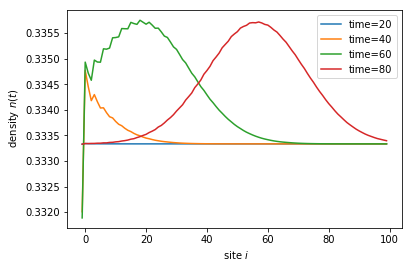
By measuring the speed of the propagating pulses without and with interaction one will find that they are propagating with Fermi velocity \(v_F\) in the first case, whereas they propagate faster with the plasmon velocity \(v_L = v_F \sqrt{1 + U / (\pi v_F)}\) in the iteracting systems. Performing a longer simulation with \(U = 0\) and \(U=10\) plotting the result as figure 1 in Ref [1] we find:

Figure 3: Electronic density \(n(i,t)\) as a function of site \(i\) for different values of time \(t\) (as indicated on the \(y\) axis) after injection of a Gaussian voltage pulse. Solid lines \(U = 10\), dashed lines \(U = 0\) (no interaction). The blue lines are linear fits with the plasmon velocity \(v_L\) (blue, solid) and with the Fermi velocity \(v_F\) (blue, dashed). The plot is analogous to figure 1 in Ref [1] and can be obtained by running the Python scripts below.

See also

Above figure can be obtained by running the three Python scripts:

plasmon_u_0_run_computation.py

plasmon_u_10_run_computation.py

plasmon_plot_results.py

2) The self-consistent Bogoliubov-deGennes / classical circuit problem

Superconducting based “quantum circuits” make one of the most advanced platform for doing quantum computation. At the classical level, these circuits are simply described by capacitances, inductances and resistors with the adjunction of one non-linear element: the (Josephson) junction between two pieces of superconductors. In some situations, it is sufficient to describe these junctions by the Josephson relation \(I = I_c \sin\phi\) but in others one needs to properly describe the fermionic quasi-particles in the superconductor. In this example, we study a Josephson junction (described by the Bogoliubov-deGennes equation) that is connected to a classical circuit (an RLC circuit, i.e. a damped harmonic oscillator) [2]. Because the current trough the junction depends on the phase difference between the two superconductors, the problem is intrinsically time dependent even if we apply a d.c. voltage difference. We will compute the current \(I(t)\) through the device when it is driven by an external electrical potential \(V_0(t)\). A schematic of the electric circuit is shown in figure 3 and the microscopic model for the Josephson junction is shown in figure 4.

Figure 3: Schematic of the classical electric circuit composed of a RLC circuit coupled to a Josephson junction. \(V_0(t)\) is the external voltage drive, \(V(t)\) is the voltage difference over the classical part and \(V_J(t)\) the voltage difference over the junction. In the RLC part, the total current \(I(t)\) is split into three contributions trought the resistance (R), capacitance (C) and inducance (L).

Figure 4: The Josephson junction is modeled with a one-dimensional tight-binding chain composed of two superconducting leads with a single normal scattering site in the center. \(\Delta\) is the superconducting gap.

Modeling of the Josephson junction (quantum part)

We simulate a short SNS junction where two semi-infinite superconducting leads (S) correspond to the region \(i < 0\) and \(i > 0\) while the normal (N) region is formed by a single site at \(i = 0\). The Hamiltonian reads [2]:

\[\begin{split}\begin{align} \hat H = \sum_{\substack{i=-\infty \\ \sigma =\uparrow,\downarrow}}^{+\infty} e^{-i\varphi_J(t)\delta_{i,-1}} \hat c^\dagger_{i\sigma}\hat c_{i+1,\sigma} + (U\delta_{i,0} - E_F) \hat c^\dagger_{i\sigma}\hat c_{i\sigma} +\sum_{i=-\infty}^{+\infty} \Delta (1-\delta_{i,0}) \hat c^\dagger_{i\uparrow}\hat c^\dagger_{i\downarrow} + h.c., \tag{16} \end{align}\end{split}\]

where \(\hat c^\dagger_{i,\sigma}\) (\(\hat c_{i,\sigma}\)) is the fermionic creation (annihilation) operator on site \(i\) and spin \(\sigma = \{ \uparrow, \downarrow \}\), the phase \(\varphi_J(t)=(e/\hbar)\int^t_0 V_J(t')dt'\) where \(V_J(t)\) is the voltage difference across the junction, which we model to take place in-between the left lead and the central site. Moreover, \(\Delta\) is the superconducting gap inside the superconductors, \(U\) is a potential barrier used to tune the transmission probability \(D\) of the junction and \(E_F\) is the Fermi energy. Such an Hamiltonian can be simulated in T-Kwant almost exactly as a usual non-superconducting Hamiltonian. Superconductivity merely doubles the number of degrees of freedom by adding an electron/hole degree of freedom on each site.

First, we rewrite the Hamiltonian in more compact form by defining the Hamiltonian matrix elements

\[\begin{align} h_{ij} = e^{-i\varphi_J(t)\delta_{i,-1}} \delta_{i,i+1} + (U\delta_{i,0} - E_F )\delta_{i,j}, \quad \Delta_{ij} = \Delta (1-\delta_{i,0}) \delta_{i,j}. \tag{17} \end{align}\]

More precisely, the above definition defines only the upper triangular part of the Hamiltonian matrix, but the lower triangular part follows trivially from hermitian symmetry. With this definition, the Hamiltonian takes the form

\[\begin{align} \hat H = \sum_{\substack{i, j=-\infty}}^{+\infty} h_{ij} (\hat c^\dagger_{i\uparrow} \hat c_{j\uparrow} + \hat c^\dagger_{i\downarrow} \hat c_{j\downarrow}) + \Delta_{ij} \hat c^\dagger_{i \uparrow} \hat c^\dagger_{j \downarrow} + \Delta^*_{ij} \hat c_{i \downarrow} \hat c_{j \uparrow} . \tag{18} \end{align}\]

Using the fermionic commutation relations, such that

\[\begin{align} h_{ij} \hat c^\dagger_{i} \hat c_{j} = \frac{1}{2} \left( h_{ij} \hat c^\dagger_{i} \hat c_{j} - h^*_{ji}\hat c_{j} \hat c^\dagger_{i} + h_{ii}\delta_{ij} \right), \tag{19} \end{align}\]

we can further rewrite the Hamiltonian into matrix form

\[\begin{align} \hat H = \sum_{\substack{i,j=-\infty}}^{+\infty} (\hat c^\dagger_{i,\uparrow}, \hat c_{i,\downarrow}) \mathbf{H}_{ij} (\hat c_{j,\uparrow}, \hat c^\dagger_{j,\downarrow})^T, \tag{20} \end{align}\]

with the Hamiltonian matrix

\[\begin{split}\begin{align} \mathbf{H}_{ij}(t) = \begin{pmatrix} h_{ij} & \Delta_{ij} \\ \Delta_{ij}^* & -h_{ij}^* \end{pmatrix} \tag{21} \end{align}\end{split}\]

At this stage, if one defines the operator \(\hat a_{i,\uparrow}^\dagger = \hat c_{i,\downarrow}\), one realizes that we’re back to a regular fermionic quadratic model, which we can solve in Tkwant directly. The only two differences introduced by superconductivity are (i) the Hamiltonian is now enlarged with a \(2\times 2\) block structure and (ii) the observables should be slightly modified (for instance the current originating from the hole sector is counted with a minus sign, see below). The matrix \(\mathbf{H}_{ij}(t)\) contains on-site terms:

\[\begin{split}\begin{align} \mathbf{H}_{ii}(t) = \begin{pmatrix} (U\delta_{i,0} - E_F ) & \Delta (1-\delta_{i,0}) \\ \Delta^* (1-\delta_{i,0}) & -(U\delta_{i,0} - E_F ) \end{pmatrix} \tag{22} \end{align}\end{split}\]

and nearest neighbour hoppings,

\[\begin{split}\begin{align} \mathbf{H}_{i+1,i}(t) = \begin{pmatrix} e^{i\varphi_J(t)\delta_{i,-1}} & 0 \\ 0 & - e^{-i\varphi_J(t)\delta_{i,-1}} \end{pmatrix} \tag{23} \end{align}\end{split}\]

Note that we have dropped a constant part stemming from the \(h_{ii}\) term, which will only lead to a shift in energy. We have also dropped the second (identical) channel with opposite spin.

For the subsequent Tkwant simulation it is customary to write the Hamiltonian matrix in \(2 \times 2\) blockmatrix form and to further decompose it as in Eq. (3) into a constant part \(\mathbf{H}_0\), a time-dependent part \(\mathbf{W}(t)\) and a self-consistent part \(\mathbf{Q}[\varphi_J(t)]\). With the help of the Pauli matrices and \(\sigma_{\alpha/\beta}\),

\[\begin{split}\begin{align} \sigma_x = \begin{pmatrix} 0 & 1 \\ 1 & 0 \end{pmatrix} , \quad \sigma_z = \begin{pmatrix} 1 & 0 \\ 0 & -1 \end{pmatrix} , \quad \sigma_\alpha = \begin{pmatrix} 1 & 0 \\ 0 & 0 \end{pmatrix} , \quad \sigma_\beta = \begin{pmatrix} 0 & 0 \\ 0 & 1 \end{pmatrix} , \tag{24} \end{align}\end{split}\]

we read off the upper triangular elements of the Hamiltonian matrix as

\[\begin{split}\begin{align} & \mathbf{H}_{0; ij} = [(U\delta_{i,0} - E_F ) \sigma_z + \Delta (1-\delta_{i,0}) \sigma_x] \delta_{i,j} + \sigma_z \delta_{i,i+1} , \quad \mathbf{W}_{ij}(t) = 0, \\ & \mathbf{Q}_{ij}[\varphi_J(t)] = [e^{-i\varphi_J(t)} \sigma_\alpha - e^{i\varphi_J(t)} \sigma_\beta - \sigma_z] \delta_{i,i+1} \delta_{i,-1}, \tag{25} \end{align}\end{split}\]

where we have taken the gap \(\Delta\) to be real. As before, the lower triangular part follows from hermitian symmetry.

To continue, we just perform the the time evolution of the manybody state in the junction. The time-dependent manybody state is described by the ensemble of time-dependent onebody Schrödinger equations, which at energy \(E\) are

\[\begin{equation} i \partial_t \psi_{\alpha E}(t, i) = \sum_j\mathbf{H}_{ij}(t) \psi_{\alpha E}(t,j) , \tag{26} \end{equation}\]

and where \(\alpha\) comprises the lead and band index and an additional spin label. The current through the junction, or more precisely from the center (site 0) to the right lead (site 1), is obtained from

\[\begin{equation} I(t) = - \left( \frac{e}{\hbar} \right) 2 i \textrm{Im} \sum_\alpha \int \frac{d E}{2 \pi} f_\alpha(E) \psi_{\alpha E}^*(t, 1) H_{1,0}(t) \sigma_z \psi_{\alpha E}(t, 0), \tag{27} \end{equation}\]

where \(f_\alpha(E) = \theta(E_{F}- E)\) and \(\theta\) is the Heaviside step function. In [2], possible boundstates have been included in the calculation, but we skip this part in order to concentrate on the self-consistent part. We now prepare the classical part of the circuit.

Electrical environment (Classical part)

The equation that describe the electromagnetic environment of the junction dues to the voltage generator and RLC circuit are just the straightforward classical equations. From the diagram of the circuit, one gets that the voltage drop \(V\) and accordingly the phases \(\varphi\) trough the classical part is

\[\begin{equation} V = V_0 - V_J, \qquad \varphi = \varphi_0 - \varphi_J. \tag{28} \end{equation}\]

Current conservation implies that

\[\begin{equation} I = I_R + I_C + I_L, \tag{29} \end{equation}\]

while the individual currents trough the resistance (R), capacitance (C) and inducance (L) are

\[\begin{equation} I_R = \frac{V}{R}, \quad I_C = C \partial_t V, \quad V = L \partial_t I_L. \tag{30} \end{equation}\]

Taking the derivative of above equation one finds

\[\begin{equation} \partial_t V = -\frac{1}{RC} V - \frac{1}{LC} \left( \frac{\hbar}{2 e} \right) \varphi + \frac{1}{c} I. \tag{31} \end{equation}\]

We define the bare oscillator frequency \(\omega_0 = 1/\sqrt{LC}\) and the quality factor \(q = R \sqrt{C/L}\) and express everything in terms of the effective energy scale \(\Delta\). In dimensionless units (denoted by a tilde) this gives

\[\begin{equation} t = \frac{\hbar}{\Delta} \tilde{t}, \quad V = \frac{\Delta}{e} \tilde{V}, \quad \omega_0 = \frac{\Delta}{\hbar} \tilde{\omega}_0, \quad I = \frac{e \Delta}{\hbar} \tilde{I}, \quad R = \frac{\hbar}{e^2} \tilde{R} \tag{32} \end{equation}\]

The differential equation for the potential becomes

\[\begin{equation} \partial_{\tilde{t}} \tilde{V} = - \frac{\tilde{\omega_0}}{q} \tilde{V} - \tilde{\omega_0}^2 \varphi + \frac{\tilde{\omega}_0 \tilde{R}}{q} \tilde{I} \tag{33} \end{equation}\]

For writing convenience we drop the tildas, nothing that all formulas in the following are expressed in dimensionless units.

Full problem

Putting everything together, the set of effective equations which must be solved self-consistently are

\[\begin{split}\begin{align} \partial_t \begin{pmatrix} \varphi \\ V \\ \psi_{\alpha E} \end{pmatrix} = \begin{pmatrix} V(t) \\ -\frac{\omega_0}{q} V(t) - \omega_0^2\varphi(t) + \frac{ \omega_0 R}{q} I(t) \\ -i(H_0 + Q(\varphi_J(t))) \end{pmatrix}. \tag{34} \end{align}\end{split}\]

Parameters

\(E_F\) gives the energy difference between the Fermi level and the bottom of the band. We scale the energy such that the Fermi level corresponds to zero thus the bottom of the band is at an energy \(E=-2\). Energies are measured in terms of the gap which is set to \(\Delta = 0.1\) and \(U = 2 \Delta\) corresponds to a junction with an intermediate transmission of \(D = 0.5\). Other parameters are \(q=20, \omega_0 = \Delta\) and \(R = 3 h / (\sqrt{2} \pi e^2)\). We will use 1 + 1 + 1 sites for the central SNS system.

We parametrize the potential \(V_0(t)\) to increase linarly from 0 to \(\Delta\) at \(t_{\rm max}\). The switching on of \(V_0(t)\) in done smoothly and we use the form

\[\begin{split}\begin{align} V_0(t) = \begin{cases} \frac{\Delta}{2 t_{\text max} - \tau} (t - \frac{\tau}{\pi} \sin(\pi t / \tau)) \,\, \, \text{if} \,\,\, t < \tau \\ \frac{\Delta}{t_{\text max} - \tau / 2} (t - \tau/2) \,\,\, \text{else.} \end{cases} \tag{35} \end{align}\end{split}\]

The phase \(\varphi_0(t)\) can be calculated explicitly by integrating \(V_0(t)\) over time:

\[\begin{split}\begin{align} \varphi_0(t) = \begin{cases} \frac{\Delta}{2 t_{\text max} - \tau} \left( \frac{t^2}{2} + \frac{\tau^2}{\pi^2} [\cos(\pi t / \tau)) - 1] \right) \,\, \, \text{if} \,\,\, t < \tau \\ \frac{\Delta}{t_{\text max} - \tau / 2} \left(\frac{t^2}{2} + \frac{t \tau}{2} + \frac{\tau^2}{4}[1 - \frac{4}{\pi^2} ]\right) \,\,\, \text{else.} \end{cases} \tag{36} \end{align}\end{split}\]

We will now solve the above equations numerically using Tkwant.

(I) Non-interacting wavefunction \(\Psi_0\)

First, we set up the non-interacting wave function.

import tkwant
import kwant
import kwantspectrum

import cmath
import numpy as np
import scipy.integrate
import scipy.interpolate
import functools
import tinyarray
import matplotlib.pyplot as plt

comm = tkwant.mpi.get_communicator()

sx = tinyarray.array([[0, 1], [1, 0]], complex)
sz = tinyarray.array([[1, 0], [0, -1]], complex)
sa = tinyarray.array([[1, 0], [0, 0]], complex)
sb = tinyarray.array([[0, 0], [0, 1]], complex)

# parameters
tmax = 10000
tau = 100
delta = 0.1
U = 2
Ef = 0
w0 = delta
dV = w0 / (2 * tmax - tau)
taupi2 = tau**2 / np.pi**2


def V0(t):
    if t < tau:
        return dV * (t - np.sin(t / tau * np.pi) * tau / np.pi)
    else:
        return 2 * dV * (t - 0.5 * tau)


def phi0(t):
    if t < tau:
        return dV * (0.5 * t**2 + (np.cos(t / tau * np.pi) - 1) * taupi2)
    else:
        return dV * (t**2 - tau * t + 0.5 * tau**2 - taupi2)


def make_SNS_system(delta, U, Ef):

    # system building
    lat = kwant.lattice.square(a=1, norbs=2)
    syst = kwant.Builder()

    # central scattering region
    onsite_N = (U - Ef) * sz
    onsite_S = - Ef * sz + delta * sx
    syst[lat(-1, 0)] = onsite_S
    syst[lat(0, 0)] = onsite_N
    syst[lat(1, 0)] = onsite_S
    syst[lat.neighbors()] = sz

    # add leads
    lead_left = kwant.Builder(kwant.TranslationalSymmetry((-1, 0)))
    lead_left[lat(0, 0)] = onsite_S
    lead_left[lat.neighbors()] = sz
    syst.attach_lead(lead_left)
    syst.attach_lead(lead_left.reversed())

    return syst, lat


# initialize the tight-binding system
syst, lat = make_SNS_system(delta, U, Ef)
syst = syst.finalized()

# set chemical potential and zero temperature (default)
occupations = tkwant.manybody.lead_occupation(chemical_potential=Ef)

# calculate the spectrum E(k) for all leads
spectra = kwantspectrum.spectra(syst.leads)

# define boundary conditions, set upper cutoff energy to Ef
boundaries = tkwant.leads.automatic_boundary(spectra, tmax, emax=Ef)


# calculate the k intervals for the quadrature
interval_type = functools.partial(tkwant.manybody.Interval, order=8,
                                  quadrature='gausslegendre')
intervals = tkwant.manybody.calc_intervals(spectra, occupations, interval_type)
intervals = tkwant.manybody.split_intervals(intervals, number_subintervals=1)

# calculate all onebody scattering states at t = 0
tasks = tkwant.manybody.calc_tasks(intervals, spectra, occupations)
psi_init = tkwant.manybody.calc_initial_state(syst, tasks, boundaries)

# set up the manybody wave function
wave_function = tkwant.manybody.WaveFunction(psi_init, tasks)

Note that we have reduced the number of intervals (number_subintervals) and the interval order (order) in above cell to allow for a fast evaluation. Numerical precise results and the figure 5 are obtained by running the Python scripts given below, which is however much more compute intensive. We can plot the system with its three central SNS sites (blue) and the semi-infinite superconducting leads (read):

kwant.plot(syst);

The Spectrum and the voltage potential are

fig, axes = plt.subplots(1, 2)
fig.set_size_inches(16, 5)

momenta = np.linspace(-np.pi, np.pi, 500)
for band in range(spectra[0].nbands):
    axes[0].plot(momenta, spectra[0](momenta, band), label='n=' + str(band))
axes[0].axhline(y=delta, color='k', linestyle='dotted', label=r'$\pm \Delta$')
axes[0].axhline(y=-delta, color='k', linestyle='dotted')
axes[0].set_xlabel(r'$k$', fontsize=16)
axes[0].set_ylabel(r'$E_n(k)$', fontsize=16)
axes[0].legend(loc=1, fontsize=16)


times = np.linspace(0, tmax)
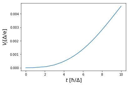
axes[1].plot(times / tmax, np.array([V0(t) for t in times]) / delta)
axes[1].set_xlabel(r'$t / t_{\rm max}$', fontsize=16)
axes[1].set_ylabel(r'$V_0(t) /\Delta$', fontsize=16)
plt.show()

(II) Operator for the current \(I(t)\) trough the junction

The current trough the junction, more precisely from the central site 0 to site 1 on the right superconducting lead, can be calculated with Kwant’s current operator:

current_operator = kwant.operator.Current(syst, onsite=sz,
                                          where=[(lat(1, 0), lat(0, 0))])

(III) Class to compute the mean-field term \(\mathbf{Q}(t)\)

To calculate the interaction contribution \(\mathbf{Q}(t)\), we implement a class called BdGPotential to solve the two remaining equations:

\[\begin{split}\begin{align} \partial_t \begin{pmatrix} \varphi \\ V \end{pmatrix} = \begin{pmatrix} V(t) \\ -\frac{\omega_0}{q} V(t) - \omega_0^2\varphi(t) + \frac{ \omega_0 R}{q} I(t) \end{pmatrix}. \tag{37} \end{align}\end{split}\]

Given the current \(I(t)\) with \(t\) in \([t_{min}, t_{max}]\) and the initial conditions \(\varphi(t_{min})\) and \(V(t_{min})\), we can solve above differential equation to obtain \(\varphi(t)\) with \(t\) in \([t_{min}, t_{max}]\). This step is implemented in the prepare() method of the class BdGPotential and we store the solution \(\varphi(t)\) in an interpolation function. The evaluate() method simply evaluates \(\varphi_j(t) = \varphi_0(t) - \varphi(t)\) at the given time \(t\) with \(t_{min} \leq t \leq t_{max}\) and returns \(\mathbf{Q}(t)\) from Eq. (25).

Our implementation to solve the differential equation (37) and to obtain the self-consistent potential Eq. (25) is

class BdGPotential:
    """A class to calculate Q(t) for the Bogoliubov-deGennes equations"""

    def __init__(self, syst, lat, w0, q, r):

        self._a = w0 / q
        self._b = w0**2
        self._c = r * w0 / q
        self._phi_init = 0
        self._v_init = 0
        self._tmin = 0
        self._tmax = 0
        self.time = []
        self.current = []
        self.phi = []
        self.v = []

        # Prepare a self-consistent hamiltonian matrix Q(t) with non-zero
        # 2x2 submatrix between site -1 and 0
        self._qt = tkwant.system.Hamiltonian(syst, hopping=(lat(0, 0), lat(-1, 0)))

    def prepare(self, current_func, tmax):
        """Pre-calculate the interaction contribution Q(t)"""
        self._tmin = self._tmax
        self._tmax = tmax

        # time grid for the solution/interpolation of the BdG differential equation
        times = np.linspace(self._tmin, self._tmax, num=4)

        def calc_rhs(tt, yy):  # right-hand-side of the BdG differential equation
            phi, v = yy
            return [v, - self._a * v - self._b * phi + self._c * current_func(tt)]

        # solve the BdG differential equation: d(phi, V) / dt = rhs
        dgl = scipy.integrate.ode(calc_rhs).set_integrator('dopri5')
        dgl.set_initial_value([self._phi_init, self._v_init], self._tmin)

        phi = [self._phi_init]
        for time in times[1:]:
            result = dgl.integrate(time)
            assert dgl.successful(), 'ode integration problem'
            phi.append(result[0])

        # save I(t), phi(t), V(t)
        # which are current, phase and voltage trought the classical circuit
        self.time.append(self._tmin)
        self.current.append(current_func(self._tmin))
        self.phi.append(self._phi_init)
        self.v.append(self._v_init)

        # initial values for the next update step
        self._phi_init = result[0]
        self._v_init = result[1]

        # interpolate phi(t) for t in [tmin, tmax]
        self._phi_func = scipy.interpolate.interp1d(times, phi, kind='cubic')

    def evaluate(self, time):
        """Return the interaction contribution Q(t) evaluated at time t in [tmin, tmax]"""
        phi_j = phi0(time) - self._phi_func(time)  # phi_j is the phase trough the junction
        ephi = cmath.exp(- 1j * phi_j) - 1
        qmat = ephi * sa - ephi.conjugate() * sb  # subblock of self-consistent matrix Q(t)
        return self._qt.get(qmat)

A crutial detail of above implementation is the construction of the \(\mathbf{Q}(t)\) matrix in the evaluate() method

ephi = cmath.exp(- 1j * phi_j(time)) - 1
qmat = ephi * sa - ephi.conjugate() * sb
qt = tkwant.system.Hamiltonian(syst, hopping=(lat(0, 0), lat(-1, 0))).get(mat)

which allows to modify \(\mathbf{Q}(t)\) self-consistently during the simulation. The above lines are equivalent to build the Kwant system in function make_SNS_system() with

def phasefunc(site1, site2, time):
    ephi = cmath.exp(- 1j * phi_j(time))
    return ephi * sa - ephi.conjugate() * sb

syst[(lat(0,0), lat(-1,0))] = phasefunc

While above construction with syst[(lat(0,0), lat(-1,0))] = phasefunc is fine for standard Tkwant simulations, this not possible for self-consistent calculations, as we need to update phi_j(time) dynamically.

In this example the mean-field potential is initialized with the parameters \(\tilde{w}_0=0.1\), \(q=20\) and \(\tilde{R} = 3 \sqrt{2}\):

bdg_potential = BdGPotential(syst, lat, w0=w0, q=20, r=3*np.sqrt(2))

(IV) Setting up the self-consistent solver

The self-consistent state is finally set up as:

sc_wavefunc = tkwant.interaction.SelfConsistentState(wave_function,
                                                     current_operator,
                                                     bdg_potential)

For the actual simulation, the wave-function wave_function_mf is propagated foreward in time:

# evolve the interacting wave function up to tmax
sc_wavefunc.evolve(time=100)
print('self-consistent update steps: ', sc_wavefunc.steps)

self-consistent update steps:  172

and we can plot the result:

v0t = [V0(t) for t in bdg_potential.time]
vj = (v0t - np.array(bdg_potential.v)) / delta
times = np.array(bdg_potential.time) * delta

plt.plot(times, vj)

plt.xlabel(r"$t\ \mathrm{[\hbar/\Delta]}$", fontsize=16)
plt.ylabel(r"$V_J \mathrm{[\Delta/e]}$", fontsize=16)
plt.plot()
plt.show()

Running the simulation until time tmax, we obtain figure 3 from Ref. [2]:

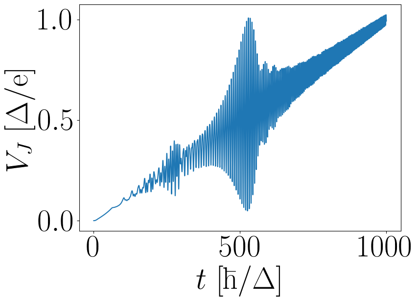
Figure 5: Voltage \(V_J(t)\) across the junction versus time \(t\) for a linear voltage ramp in \(V_0(t)\). The figure is analogous to figure 3 in Ref [2] and can be obtained by running the Python scripts below.

See also

Above figure can be obtained by running the two Python scripts:

bdg_junction_run_computation.py

bdg_junction_plot_results.py

3) Landau-Lifshitz-Gilbert equation study for spin dynamics

The third example that we consider is the interplay between the electronic and magnetic degrees of freedom in a spintronics system. The transport electrons feel the magnetization as an effective spin dependent potential (sd coupling) and in return exert a spin torque on the magnetization. The dynamics of the magnetization is treated classically at the Landau-Lifshitz-Gilbert (LLG) level. Self-consistent Tkwant can solve the self-consistent Schrödinger-LLG problem. The problem we consider corresponds to Ref. [3]. The Hamiltonian for the electronic part is

\[\begin{equation} H = \sum_{<ij>} \gamma_{ij} c^\dagger_{i} c_{j} -J_{sd} \sum_{i} c^\dagger_{i} \mathbf{\sigma} \cdot \mathbf{M}_i(t) c_{i}. \tag{38} \end{equation}\]

where \(c^\dagger_{i} = (c^\dagger_{i \uparrow}, c^\dagger_{i\downarrow})\) is the fermionic creation respectively \(c_{i\sigma}\) the annihilation operator on site \(i\), \(\gamma_{ij}\) the hopping term, \(\mathbf{\sigma} = (\sigma_x, \sigma_y, \sigma_z)^T\) is the vector of Pauli matrices, \(J_{sd}\) the strength of the exchange interaction and \(\mathbf{M}_i(t)\) the local magnetization. The magnetic energy is

\[\begin{equation} \mathcal{H} = -J \sum_{<ij>} \mathbf{M}_i \cdot \mathbf{M}_j - \mu_M \sum_{i} \mathbf{M}_i \cdot \mathbf{B}^i_{\text ext}(t) - K \sum_{i} (M^x_i)^2 - J_{sd} \sum_{i} \langle \mathbf{s} \rangle^i \cdot \mathbf{M}_i \tag{39} \end{equation}\]

where \(J\) is the Heisenberg exchange coupling parameter, \(\mathbf{B}^i_{\text ext}\) the external magnetic field, \(K\) the magnetic anisotropy in the x direction, \(\mu_M\) the magnitude of the local magnetic moment and \(\langle \mathbf{s} \rangle^i\) the nonequilibrium electronic spin density on site \(i\). The magnetization can be computed from the LLG equation (here for simplicity we neglect the damping term but note that the conducing electrons will generate an effective damping in the dynamics),

\[\begin{equation} \frac{\partial \mathbf{M}_i(t)}{\partial t} = - g \mathbf{M}_i(t) \times \mathbf{B}^{\text eff}_{i}(t), \qquad \mathbf{B}^{\text eff}_{i}(t) = - \frac{1}{\mu_M} \frac{\partial \mathcal{H}}{\partial \mathbf{M}_i(t)}. \tag{40} \end{equation}\]

In the following we will focus on the situation of a single interacting site \(i_0 = 0\). The effective magnetic field follows from Eqs. (39) and (40) as

\[\begin{equation} \mathbf{B}^{\text eff}_{i_0}(t) = \mathbf{B}_{i_0, \text ext}(t) + 2 K/\mu_M M^x_{i_0}(t) \mathbf{e}_x + J_{sd} /\mu_M \langle \mathbf{s} \rangle_{i_0} \tag{41} \end{equation}\]

and Hamiltonian matrix follows from Eq. (38) as

\[\begin{equation} H_{ij} = \gamma_{ij} - J_{sd} \mathbf{\sigma} \mathbf{M}_{i_0}(t) \delta_{i, i_0} \delta(t) \tag{42} \end{equation}\]

The elements of the Hamiltonian matrix Eq. (3) are therefore: \(H_0 = \gamma_{ij}\), \(W(t) = 0\) and the mean-field term is

\[\begin{equation} \mathbf{Q}(t) = - J_{sd} \mathbf{\sigma} \cdot [\mathbf{M}_{i_0}(t) - \mathbf{M}_{i_0}(t=0)] \delta_{i, i_0} \delta(t) . \tag{43} \end{equation}\]

Parameters

We parametrize the external magnetic field as

\[\begin{equation} \mathbf{B}_{i, \text ext}(t) = B_0 \cos(\omega t) \vec{e}_z \delta_{i,0} \tag{44} \end{equation}\]

and define the variables \(k \equiv K/\mu_M\) and \(jds = J_{sd} /\mu_M\). Moreover, we define the system to have only three sites, the hopping term \(\gamma_{ij} = -1\) is only nonzero for neighboring sites and \(M(t)\) is considered only on the central site \(i_0\).

(I) Non-interacting wavefunction \(\Psi_0\)

The noninteracting system is defined by

import tkwant
import kwant
import kwantspectrum

import tinyarray
import functools
import numpy as np
import scipy.integrate, scipy.interpolate, scipy.sparse
import matplotlib.pyplot as plt


s0 = tinyarray.array([[1, 0], [0, 1]])
sx = tinyarray.array([[0, 1], [1, 0]])
sy = tinyarray.array([[0, -1j], [1j, 0]])
sz = tinyarray.array([[1, 0], [0, -1]])


def make_spin_chain(L=3):

    # system building
    lat = kwant.lattice.square(a=1, norbs=2)
    syst = kwant.Builder()

    # central scattering region
    syst[(lat(x, 0) for x in range(L))] = sz
    syst[lat.neighbors()] = -sz

    # add leads
    lead_left = kwant.Builder(kwant.TranslationalSymmetry((-1, 0)))
    lead_left[lat(0, 0)] = sz
    lead_left[lat.neighbors()] = -sz
    syst.attach_lead(lead_left)
    syst.attach_lead(lead_left.reversed())

    return syst, lat


syst, lat = make_spin_chain()
syst = syst.finalized()

times = np.arange(0, 100, 1.0)

# calculate the spectrum E(k) for all leads
spectra = kwantspectrum.spectra(syst.leads)

# estimate the cutoff energy Ecut from T, \mu and f(E)
# All states are effectively empty above E_cut
occupations = tkwant.manybody.lead_occupation(chemical_potential=0)

# define boundary conditions
bdr = tkwant.leads.automatic_boundary(spectra, tmax=max(times), emax=0)

# calculate the k intervals for the quadrature
interval_type = functools.partial(tkwant.manybody.Interval, order=4,
                                  quadrature='gausslegendre')
intervals = tkwant.manybody.calc_intervals(spectra, occupations, interval_type)
intervals = tkwant.manybody.split_intervals(intervals, number_subintervals=1)

# calculate all onebody scattering states at t = 0
tasks = tkwant.manybody.calc_tasks(intervals, spectra, occupations)
psi_init = tkwant.manybody.calc_initial_state(syst, tasks, bdr)

# set up the manybody wave function
wave_function = tkwant.manybody.WaveFunction(psi_init, tasks)

Note that the interval order and the number of subinterval, aka order and number_subintervals, were lowered to speed up the simulation for the tutorial. For numerically accurate results, the values must be choosen much higher.

(II) Operator to compute the spin density

The spin density can be calculate with the standard kwant.operator.Density operator. As we need all three components \(x,y, z\), we need to write a small wrapper class which returns the three components of the spin density \(\langle \mathbf{s} \rangle^i = (\langle \mathbf{s} \rangle^x_i, \langle \mathbf{s} \rangle^x_i, \langle \mathbf{s} \rangle^x_i)^T\) on site \(i\):

class SpinDensity:
    """Calculate the spin density vector

    An instance of this class can be called like a kwant operator.
    """
    def __init__(self, syst, where=None):
        self.rho_sx = kwant.operator.Density(syst, sx, where=where)
        self.rho_sy = kwant.operator.Density(syst, sy, where=where)
        self.rho_sz = kwant.operator.Density(syst, sz, where=where)
    def __call__(self, bra, ket=None, args=(), *, params=None):
        return np.array([self.rho_sx(bra), self.rho_sy(bra), self.rho_sz(bra)])

spindens_operator = SpinDensity(syst, where=[lat(1, 0)])
spin_density0 = wave_function.evaluate(spindens_operator, root=None)

(III) Class to compute the mean-field term \(\mathbf{Q}(t)\)

The self-consistent potential \(\mathbf{Q}(t)\) in Eq. (43) is implemented as:

class B_ext:
    """External time-dependent magnetic field"""
    def __init__(self, omega, b0):
        self._omega = omega
        self._b0 = b0
    def __call__(self, time):
        return self._b0 * np.cos(self._omega * time)


class LLG_Potential:
    """A class to calculate Q(t) for the Landau-Lifshitz-Gilbert equations"""

    def __init__(self, syst, lat, b_ext, g, k, jds, spin_density0, m0=(0, 0, 0), time0=0):

        self._b_ext = b_ext
        self._g = g
        self._k = k
        self._jds = jds
        self._spin_density0 = spin_density0
        self._m0 = m0
        self._tmin = time0
        self._tmax = time0
        self._ucount = 0

        # to store the magnetization m(t) and timestep history
        self.magnet = [m0]
        self.times = [0]

        self._qt = tkwant.system.Hamiltonian(syst, site=lat(1, 0))

    def prepare(self, spin_density_func, tmax):
        """Pre-calculate the interaction contribution Q(t) for t in [tmin, tmax]"""

        self._ucount += 1
        self._tmin = self._tmax
        self._tmax = tmax

        # time grid for the solution/interpolation of the LLG differential equation
        times = np.linspace(self._tmin, self._tmax, num=4)

        def calc_rhs(tt, mvec):  # right-hand-side of the LLG differential equation
            mx, my, mz = mvec
            bz = self._b_ext(tt)
            svec = spin_density_func(tt) - self._spin_density0
            mb = (0, my * bz, - mx * bz)  # M x B_ext
            mmx = (- self._k * mx * my, 0, self._k * mx * mz)  # k * M x M_x
            ms = self._jds * np.cross(mvec, svec)  # J_ds * M x <s>
            return - self._g * np.array([mmx[0] + ms[0], mb[1] + ms[1], mb[2] + mmx[2] + ms[2]])

        # solve the BdG differential equation: d(phi, V) / dt = rhs
        dgl = scipy.integrate.ode(calc_rhs).set_integrator('dopri5')
        dgl.set_initial_value([self._m0[0], self._m0[1], self._m0[2]], self._tmin)

        magnetization = [self._m0]  # m(t) at t=tmin
        for time in times[1:]:
            result = dgl.integrate(time)
            assert dgl.successful(), 'ode integration problem'
            magnetization.append(result)

        # store m(t) and the timesteps
        self.times.append(self._tmin)
        self.magnet.append(self._m0)

        # store m(t) at t=tmax which will be the initial values for the next update step
        self._m0 = tuple(result)

        # interpolate m(t) for t in [tmin, tmax]
        self._mt = scipy.interpolate.interp1d(times, np.array(magnetization).T, kind='cubic')

    def evaluate(self, time):
        """Return the interaction contribution Q(t) evaluated at time *t*"""
        #  assert self._tmin <= time <= self._tmax  # consistency check
        mx, my, mz = self._mt(time)
        mx0, my0, mz0 = self.magnet[0]
        m_sigma = - self._jds * ((mx - mx0) * sx + (my - my0) * sy + (mz - mz0) * sz)
        return self._qt.get(m_sigma)

We use the following parameters for the simulation:

b_ext = B_ext(omega=1, b0=1)

llg_potential = LLG_Potential(syst, lat, b_ext, g=1, k=1, jds=1,
                              spin_density0=spin_density0, m0=(0.1, 0, 0))

(IV) Setting up the self-consistent solver

The self-consistent solver is initialized with

sc_wavefunc = tkwant.interaction.SelfConsistentState(wave_function,
                                                     spindens_operator,
                                                     llg_potential)

and the numerical solution performed in

sc_wavefunc.evolve(time=2)
print('self-consistent update steps: ', sc_wavefunc.steps)


plt.plot(llg_potential.times, llg_potential.magnet)
plt.xlabel(r'time $t$')
plt.ylabel(r'magnetization $m(t)$')
plt.gca().legend((r'$m_x$', r'$m_y$', r'$m_z$'))
plt.show()

self-consistent update steps:  404

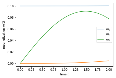
Running such a simulation for a longer times one should be able to reproduce the results from Ref. [3]. For such a simulation, also the numbers for order and number_subintervals would need to be increased to get numerically accurate results.

2.9.6. Advanced settings

Below are some additional details on the internals of self-consistent Tkwant.

Accuracy of the self-consistent updates and adaptive stepsize control

The update of the self-consistent potential is done adaptively depending on the estimated extrapolation error. For a time interval \([t_{\text{min}}, t_{\text{max}}]\), the error \(err\) is estimated from the extrapolated mean-field operator value Eq.(5) as:

\[\begin{equation} err = \text{max}|\tilde{y}(t_{\text{max}}) - y (t_{\text{max}})|. \tag{45} \end{equation}\]

The accuracy of this extrapolation can be changed via the two arguments atol and rtol of the class tkwant.interaction.SelfConsistentState. The default value of the parameters atol and rtol has been chosen to be rather conservative in terms of the tolerated error (see the code for the current default values) and the code can sometimes be significantly accelerated by relaxing these values a little. Changing these values also provides a direct way to check the convergence of the extrapolation scheme.

sc_wavefunc = tkwant.interaction.SelfConsistentState(wave_function, density_operator,
                                                     hartree_potential, rtol=1e-5, atol=1e-5)

Using smaller (more precise) value of atol and rtol will force tkwant.interaction.SelfConsistentState to update the self-consistent potential more often to meet the required accuracy. The stepping is done adaptively with the class tkwant.interaction.AdaptiveStepsize, but one can also change the behavior of this class. The initial stepsize for instance can be changed via:

import functools as ft

# pre-bind new minimal stepsize to the adaptive stepsize control
tau = ft.partial(tkwant.interaction.AdaptiveStepsize, tau_min=1e-4)

sc_wavefunc = tkwant.interaction.SelfConsistentState(wave_function, density_operator,
                                                     hartree_potential, tau=tau)

Alternatively, one can switch of the adaptive stepsize completely and use a constant stepping instead. Here we use a constant stepsize of \(\tau=0.01\) for the self-consistent updates:

sc_wavefunc = tkwant.interaction.SelfConsistentState(wave_function, density_operator,
                                                     hartree_potential, tau=0.01)

Mean-field extrapolation

According to Eq. (7), the expectation value \(y (t)\) must be extrapolated to future times, in order to solve the Schödinger equation. When the true expectation value \(y(t)\) is evaluead at a given timestep, the extrapolation function \(\tilde{y}(t)\) is updated. Different ways to perform the extrapolation are possible. They are shown here with a simple scalar model function \(y(x)\), where \(x\) takes the role of time \(t\) in our concrete physical usecase. The extrapolated function is denoted as \(\tilde{y}(x)\) (which corresponds to yt in the prepare() method of the class MyMeanFieldPotentialQ()). The update stepsize is tau and is taken as constant for simplicity.

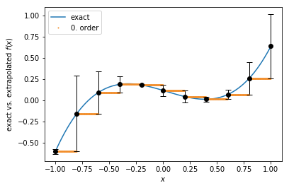
0. order extrapolation

While conceptionally very simpe, the 0.order extrapolation function has steps at the update times:

def f(x):
    return (x - 0.2)**3 + 0.5 * (x - 0.5)**2

tau = 0.2
sample_pts = np.round(np.linspace(-1, 1, 1001), 4)
update_pts = np.asarray([np.round(-1 + tau * i, 4) for i in range(11)])

plt.plot(sample_pts, f(sample_pts))

ft = tkwant.interaction.Extrapolate(f(-1.01), 0.01, order=0, x0=-1.01)

for x in sample_pts:
    if x in update_pts:
        error = ft.add_point(x, f(x))
        ft.set_stepsize(tau)
        plt.errorbar(x, f(x), yerr=abs(error), fmt='ok', ecolor='k', elinewidth=1, capsize=4)
    plt.plot(x, ft(x), 'o', c='#f28e2b', markersize=1)

plt.gca().legend(('exact','0. order'))
plt.xlabel(r'$x$')
plt.ylabel(r'exact vs. extrapolated $f(x)$')
plt.show()

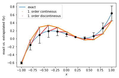
1. order extrapolation

Two different ways are shown here to perform a linear extrapolation: With standard linear extrapolation, the extrapolated function \(y(x)\) has again discontineous steps at the update points. Contineous linear extrapolation, which is also the default method, has no jumps in the extrapolation function when the potential is updated, but coincides with the discontineous 1. order extrapolation with the point at the future update.

plt.plot(sample_pts, f(sample_pts))

x0 = -1.01
y0 = f(x0)

ft = tkwant.interaction.Extrapolate(y0, 0.01, order=1, x0=x0)

for x in sample_pts:
    if x in update_pts:
        error = ft.add_point(x, f(x))
        ft.set_stepsize(tau)
        x1, y1 = x, f(x)
        dy = (y1 - y0) / (x1 - x0)
        x0, y0 = x1, y1
        plt.errorbar(x, y1, yerr=abs(error), fmt='ok', ecolor='k', elinewidth=1, capsize=4)
    plt.plot(x, ft(x), 'o', c='#f28e2b', markersize=1)
    plt.plot(x, y0 + (x - x0) * dy, 'o', c='#e15759', markersize=1)

plt.gca().legend(('exact','1. order contineous', '1. order discontineous'))
plt.xlabel(r'$x$')
plt.ylabel(r'exact vs. extrapolated $f(x)$')
plt.show()

Changing the extrapolation order

The extrapolation order can be changed in the following way:

# pre-bind new order to the extrapolate
import functools
extrapolate = functools.partial(tkwant.interaction.Extrapolate, order=0)

# set up the self-consistent interacting manybody wave function with a new extrapolator
sc_wavefunc = tkwant.interaction.SelfConsistentState(wave_function, density_operator,
                                                     hartree_potential,
                                                     extrapolator_type=extrapolate)

2.9.7. References

[1] T. Kloss, J. Weston, and X. Waintal, Transient and Sharvin resistances of Luttinger liquids, Phys. Rev. B 97,165134 (2018).

[2] B. Rossignol, T. Kloss, and X. Waintal, Role of Quasi-particles in an Electric Circuit with Josephson Junctions, Phys. Rev. Lett. 122, 207702 (2019).

[3] U. Bajpai and B. K. Nikolic, Time-retarded damping and magnetic inertia in the Landau-Lifshitz-Gilbert equation self-consistently coupled to electronic time-dependent nonequilibrium Green functions, Phys. Rev. B 99, 134409 (2019).

[4] T. Kloss, J. Weston, B. Gaury, B. Rossignol, C. Groth and X. Waintal, Tkwant: a software package for time-dependent quantum transport, New J. Phys. 23, 023025 (2021).