2.12. Boundary conditions

To simulate open quantum systems with tkwant, modes that are propagating from a central scattering region into a lead are not supposed to return into the scattering region anymore. This behavior is ensured by special boundary conditions that we have to provide when solving the time-dependent Schödinger equation. No additional boundary conditions must be provided for closed systens, as the wavefunction is by definition zero at the system border.

The two high-level solver routines onebody.ScatteringStates() and manybody.States() calculate internally the required boundary contitions. This happens e.g. in the open system example Evolution of a scattering state under a voltage pulse in a quantum dot, when the solver is initialized:

psi = tkwant.onebody.ScatteringStates(syst, energy=1., lead=0, tmax=200)[0]

One can prevent the solver to use the internal default boundaries but pass own boundary conditions to the solver that will be used instead:

boundaries = tkwant.leads.automatic_boundary(syst.leads, tmax=200)
psi = tkwant.onebody.ScatteringStates(syst, energy=1., lead=0,
                                      boundaries=boundaries)[0]

This is a good way to change default parameters and precalculating boundaries is also mandatory to construct wave functions using the low level approach via onebody.WaveFunction(). We will show in this tutorial how boundary conditions work and how to calculate and analyse them.

See also

An full example script showing how default boundaries are changed can be found in Alternative boundary conditions.

2.12.1. Basic formalism

We will use the approach developed in Ref. [1] employing an imaginary potential, to construct so-called absorbing boundary conditions. This tutorial will illustrate how to set absorbing boundary conditions in the general case. For advanced users, it also shows how to set up boundary conditions by hand and how to analyze them, if desired.

Absorbing boundary conditions are not ideal but have some spurious reflection. We define the reflection coefficient \(r\) by

\[\psi(x) = e^{i k x} + r e^{-i k x} .\]

The first term is the initial propagation of the plane wave \(\psi(x)\), whereas the second term is the reflected part. The reflection coefficient \(r\) ranges between zero (no reflection) and one (total reflection).

In the general case, different modes (indexed by \(\alpha\)) with corresponding wave vector \(k_{\alpha}\) are open for a given energy \(E\). We write the reflection as

\[\psi_\alpha(x) = e^{i k_\alpha x} + r_{\alpha} e^{-i k_\alpha x} .\]

To obtain the full lead reflection, we have to sum over all open modes:

\[r = \sum_\alpha |r_{\alpha}|\]

2.12.2. A minimal example

We start with a simple example and construct boundary conditions for a lead lead which is three sites wide. The Hamiltonian of the system is

\[\hat{H}(t) = \sum_{ij} 2 |i,j \rangle \langle i,j | - (|i+1,j \rangle \langle i,j | + |i,j \rangle \langle i+1,j | + |i,j + 1 \rangle \langle i,j | + |i,j \rangle \langle i,j + 1 | )\]

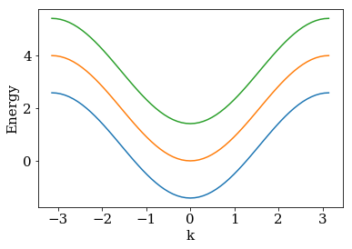
The system is translationally invariant in the direction of index i (which takes values from \(-\infty\) to \(\infty\)) and runs in j direction over the three sites 0, 1 and 2. Let us first construct the lead with kwant and show its spectrum with three bands in the first Brillouin zone.

import tkwant
import kwant

# create lead
def make_lead(W=3):
    lat = kwant.lattice.square(a=1, norbs=1)
    lead = kwant.Builder(kwant.TranslationalSymmetry((-1, 0)))
    lead[(lat(0, y) for y in range(W))] = 2
    lead[lat.neighbors()] = -1
    return lead.finalized()

lead = make_lead()
kwant.plotter.bands(lead);

In a realistic model one has to imagine this lead attached to some central scattering region that we like to study by a tkwant simulation. To make the steps more explicit however, we will concentrate on the lead only in this tutorial.

Automatic boundary conditions

The easiest way to construct boundary conditions is to use the fully automatic routine automatic_boundary. We only have to provide the lead and a maximal simulation time tmax, that we have to fix in advance for the subsequent tkwant simulation.

boundary = tkwant.leads.automatic_boundary(lead, tmax=10000)

The boundary condition boundary is ready to use with the tkwant solvers. It is intended to provide an optimal boundary for our system. In the case that the system has several leads, one has to provide a sequence of boundary condtions to the solver, a boundary condition per lead. The automatic_boundary can take a sequence of leads as an input parameter and returns automatically a sequence of boundaries, as in the initial example.

Changing default values

Without further arguments automatic_boundary, the reflection r is smaller than a given default value. The value can be changed by the keyword refl_max.

boundary = tkwant.leads.automatic_boundary(lead, tmax=10000, refl_max=1E-10)

If we have upper (like the Fermi energy for low temperatures) and or lower energy cutoffs, we can pass it to the routine with the keyword emax and emin. This might result in a computationally more efficient boundary condition. If we simulate only modes between the energies 0 and 1 we could write:

boundary = tkwant.leads.automatic_boundary(lead, tmax=10000, emin=0, emax=1)

WARNING:tkwant.leads:1318:rank=0: could not find maximal curvature value for spectrum within emin=0, emax=1

WARNING:tkwant.leads:1926:rank=0: problem to analyse spectrum for boundary conditions: unable to find max curvature point of the spectrum

This should be the standard way to construct boundary conditions that is sufficient in most cases. If the algorithm in routine automatic_boundary fails, or the performance of the obtained boundary condition is too low and we like to optimize by hand, we provide tools to set up and analyze boundary conditions by hand. They are discussed in the two following paragraphs.

2.12.3. How do tkwant boundary conditions work

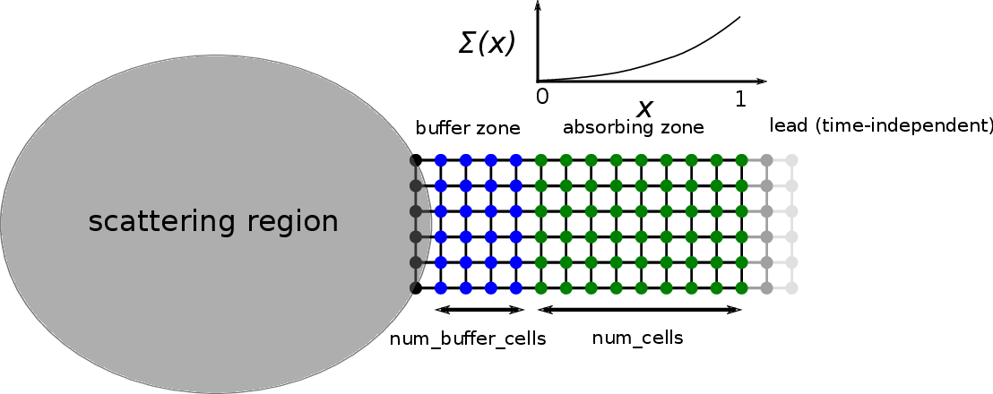
Technically, the tkwant boundary conditions work by additional cells, that are inserted between the scattering region and the (time independent) lead. Two different types of cells can be added. In the buffer zone, which is the first zone connected to the scattering region (colored in blue below), num_buffer_cells with the lead hamiltonian are added. Here in our example, num_buffer_cells = 3 and the lead width is 6. In the buffer zone, the modes coming from the system simply continue to propagate into the lead during the simulation. A second zone is the so-called absorbing zone (colored in green below), which is in our example is num_absorb_cells = 9 cells long. An absorbing potential \(i \Sigma(x)\) is added to the Hamiltonian in order to create damping and absorb propagating waves. For convenience, we will often skip the imaginary unit \(i\) in front of the absorbing potential \(\Sigma(x)\). The first discrete absorbing cell corresponds to \(x = 0\) of the (continous) argument for \(\Sigma(x)\), whereas \(x = 1\) corresponds to the last absorbing cell on the right, that is facing the time-independent lead (shown in grey). Having present only buffer, absorbing, or both zones, we distinguish three types of boundary conditions, that we discuss in the following.

Simple boundary conditions

One can also set up boundary conditions by hand. The simplest boundary condition consists in adding num_buffer_cells additional cells that are explicitly taken into account in the time-dependent simulation, in between the scattering region and the lead. This type of boundary conditions can be obtained via:

boundary = tkwant.leads.SimpleBoundary(num_buffer_cells=1000)

Up to the simulation time of 2 * num_buffer_cells / vmax where vmax is the maximal velocity of a mode in the lead, very little reflection is comming from the lead where this boundary is used. The disadvantage of this type of boundary condition is that it is becomes very inefficient for long simulation times, as the number of added lead cells num_buffer_cells increases linearly with the maximal time tmax.

Monomial absorbing boundary conditions

An often much better approach is to use absorbing boundary conditions, that add an imaginary background potential \(\Sigma(x)\) onto the num_absorb_cells additional lead cells, in order to absorb waves that are propagating into the lead. The specific form of a monomial imaginary potential

\[\Sigma(x) = (n + 1) A x^n ,\]

was explored in Ref. [1]. This boundary can easily set up by writing:

num_absorb_cells = 400
boundary = tkwant.leads.MonomialAbsorbingBoundary(num_absorb_cells, strength=10, degree=4)

where n is the degree of the polynomial and A corresponds to the strength. The absorbing boundary condition has the advantage that no maximal time has to be choosen in advance of the simulation. In addition, it has a much better scaling behavior, as the number of explicit lead cells num_absorb_cells does not scale linearly with the simulation time as before. The disadvantage of this approach is that the choice of the three parameters, as the one we took above, is rather heuristic. As absorbing boundary conditions will always lead to a hopefully small, but finite reflection from the lead, this is especially unpleasant as we have no explicit control of the error in advance. We will show in the later section however how to estimate the lead reflection for a given choice of the parameters, respectivelly a generic imaginary potential \(\Sigma(x)\).

As a side remark, let us state that the routine automatic_boundary employs an algorithm to estimate an optimal choice of the monomial parameters degree, strength and degree (and also additional buffer cells num_buffer_cells, that will be discussed below), such that the reflection stays below a given value refl_max. It then returns either a MonomialAbsorbingBoundary or a SimpleBoundary condition, depending on which one is computationally more efficient.

General absorbing boundary conditions

Finally, one may choose an arbitrary static imaginary potential \(\Sigma(x)\) to construct an absorbing boundary condition. The argument domain is \(0 \leq x \leq 1\). Having num_total_cells = num_absorb_cells + num_buffer_cells lead cells, \(x = 0\) corresponds to the first lead cell (index 0) that is connected to the scattering region respectively to the buffer, if num_buffer_cells > 0, whereas \(x = 1\) corresponds to the the last lead cell (index num_total_cells - 1). The specific form of monomial potential used above can be simply recovered by setting:

def my_imaginary_potential(x):
    return 50 * x**4

boundary = tkwant.leads.GenericAbsorbingBoundary(num_absorb_cells, my_imaginary_potential)

2.12.4. Lead reflection analysis

Basic analysis

The most obvious way to study unintended reflections of an absorbing lead is to perform the time dependent tkwant simulation with different boundary conditions and check a posteriori the observables afterwards for spurious reflections. Alternatively, as a tkwant simulations are computationally demanding, one can perform an a priori estimate of the lead reflection with an imaginary potential \(\Sigma(x)\) by a static kwant calculation. The absorbing potential can then be tuned to meet a desired maximal reflection.

The AbsorbingReflectionSolver calculates the reflection for an absorbing lead of length num_absorb_cells with the imaginary potential \(\Sigma(x)\). Calling an instance of AbsorbingReflectionSolver for a given energy energies, it returns the reflection, momenta and velocities of all open modes at this energy.

reflection_solver = tkwant.leads.AbsorbingReflectionSolver(lead, num_absorb_cells,
                                                           my_imaginary_potential)
refl, k, vel = reflection_solver(energies=0.5)
print('reflection = {}'.format(refl))
print('momenta = {}'.format(k))
print('velocities = {}'.format(vel))

reflection = [4.5107e-05 2.8341e-07]
momenta = [1.5279 0.7227]
velocities = [1.9982 1.3229]

Advanced analysis

As the number of open modes and also their ordering might change with the energy, it becomes tedious to analyze a more complicated spectrum with the AbsorbingReflectionSolver. A more convenient way is to use the AnalyzeReflection class. Calling an instance of this class with a momentum k and the band index band, we obtain the reflection, energy and velocity of the corresponding mode

analyze_reflection = tkwant.leads.AnalyzeReflection(lead, num_absorb_cells,
                                                    my_imaginary_potential)
refl, energy, vel = analyze_reflection(k=0.2, band=1)
print('reflection = {:10.4e}, energy = {:6.4f}, velocity = {:6.4f}'.format(refl, energy, vel))

reflection = 2.8802e-08, energy = 0.0399, velocity = 0.3973

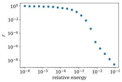
Moreover, we expect strong reflections around the local dispersion minima or maxima. The around_extremum method of the AnalyzeReflection provides an easy way to examine these regions. Note that plots very similar to the one in Ref. [1] can be obtained easily in this way. In the figure, “relative energy” denotes \(E_{n=1}(k) - E_{n=1}(0)\). The blue dots around the minima of the middle band are the one for which we calculated the reflection.

import matplotlib.pyplot as plt

# helper routine for log plots
def log_plot(x, y, xlabel, ylabel=r'$r$', show=True):
    plt.plot(x, y, 'o')
    plt.xscale('log')
    plt.yscale('log')
    plt.xlabel(xlabel)
    plt.ylabel(ylabel)
    if show:
        plt.show()

# reflection around dispersion minimum of band 1
refl, e, vel, k, e0, k0 = analyze_reflection.around_extremum(kmin=-0.3, kmax=0.3,
                                                             band=1)
log_plot(e, refl, xlabel='relative energy')

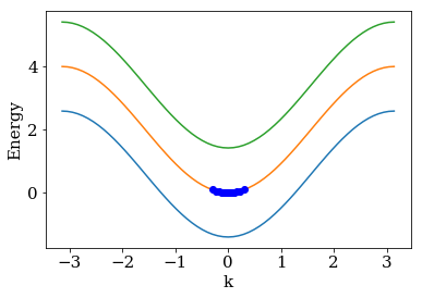
# lead dispersion and the location of the points for that we calculated the reflection
kwant.plotter.bands(lead, show=False)
plt.plot(k + k0, e + e0, 'ob')
plt.show()

We can get rid of the slow modes with high reflection by adding an additional buffer zone in between the scattering region and the absorbing region. Adding num_buffer_cells to the lead and plotting the reflection against the velocity, the modes with a velocity smaller than buffer_vmax will not lead to reflection as they stay into the buffer zone (the part on the left of the horizonal black dashed line in the figure below). Only the modes with velocity higher than buffer_vmax will be surpass the buffer zone and reflected in the absorbed region (the part on the right of the horizonal black dashed line in the figure below).

num_buffer_cells, tmax = 600, 10000
buffer_vmax = 2 * num_buffer_cells / tmax
plt.plot([buffer_vmax] * 2, [min(refl), max(refl)], 'k--')
log_plot(vel, refl, xlabel=r'$v$')

2.12.5. An advanced example with “nasty modes”

We will consider a more involved problem with hybidized bands. In contrast to the former simple problem, the small band gaps at the avoided crossings lead to pretty high curvatures in the local dispersion extrema. This means that we get fast modes with relatively low excitation energies, measured from the local extrema, such that these modes travel fast through the buffer but are also strongly reflected from the absorbing potential \(\Sigma(x)\).

We first plot the spectrum and also mark two modes that have different requirements for the monomial parameter optimization of the boundary algorithm:

One mode with high curvature and low excitation energy. The low energy of this mode means that it is strongly reflected at the imaginary potential, so the strenght parameter needs to be small. In contrast to the former problem however, the low-energy mode propagates fast due to the high curvature. It is therfore not cut off by the buffer zone as in the previous example. A second mode with high velocity and high excitation energy. This mode is not supposed to be captured by the buffer zone, but needs a strong enough imaginary potential with a large strength parameter to be well absorbed. The reflection at the absorbing potential plays a much weaker role than for the low energy mode.

import numpy as np
import tinyarray as ta
import kwantspectrum

# definition of the lead
def hybrid_lead(Delta=0.1, alpha=0.3, Ez=0.5, Ef=0.7):

    s0 = [[1, 0], [0, 1]]
    sx = [[0, 1], [1, 0]]
    sy = [[0, -1j], [1j, 0]]
    sz = [[1, 0], [0, -1]]
    sz0 = ta.array(np.kron(sz, s0), complex)
    szx = ta.array(np.kron(sz, sx), complex)
    s0z = ta.array(np.kron(s0, sz), complex)
    sx0 = ta.array(np.kron(sx, s0), complex)

    def onsite_S(*x):
        return (2 - Ef) * sz0 + Ez * s0z + Delta * sx0

    def hopping(*x):
        return -sz0 - 1j * alpha * szx

    lat = kwant.lattice.square(norbs=4)
    lead = kwant.Builder(kwant.TranslationalSymmetry((-1, 0)))
    lead[lat(0, 0)] = onsite_S
    lead[lat.neighbors()] = hopping
    return lead

lead = hybrid_lead().finalized()
fermi_energy = 0

# plot the dispersion
spectrum = kwantspectrum.spectrum(lead)
k1, k2 = -1.80350, -1.29787
vmax = np.abs(spectrum(k1, band=1, derivative_order=1))
gmax = np.abs(spectrum(k2, band=1, derivative_order=2))
print('max velocity = {:6.4f}, max curvature = {:6.4f}'.format(vmax, gmax))

kwant.plotter.bands(lead, show=False)
plt.plot([-np.pi, np.pi], [fermi_energy] * 2, 'k--')
plt.plot(k1, spectrum(k1, band=1), 'or', label='max velocity')
plt.plot(k2, spectrum(k2, band=1), 'ob', label='max curvature in extremum')
plt.legend()
plt.show()

max velocity = 2.0436, max curvature = 42.5971

Estimate optimal monomial parameters

We can check the monomial parameters that automatic_boundary proposes from the returned boundary instance:

boundary = tkwant.leads.automatic_boundary(lead, tmax, refl_max=1E-5,
                                           emax=fermi_energy)
print('num_absorb_cells = {b.num_absorb_cells}, strength = {b.strength:6.4f}, '
      'degree = {b.degree}, num_buffer_cells = {b.num_buffer_cells}'
      .format(b=boundary[0]))

num_absorb_cells = 1861, strength = 109.0439, degree = 6, num_buffer_cells = 2126

Alternatively, we can call directly the parameter estimate routine, that is internally used by automatic_boundary to obtain the monomial parameters:

tmp = tkwant.leads._monomial_parameter_estimate(spectrum, tmax,refl_max=1E-5,
                                                degree=6, emax=fermi_energy)
num_absorb_cells, strength, num_buffer_cells, *_ = tmp

print('num_absorb_cells = {}, strength = {:6.4f}, num_buffer_cells = {}'
      .format(num_absorb_cells, strength, num_buffer_cells))

num_absorb_cells = 1861, strength = 109.0439, num_buffer_cells = 2126

Reflection of the nasty modes

As before, we can now analyze the refection of the lead with the specific monomial potential. We will use however the AnalyzeReflectionMonomial class, which has a similar functionality as the AnalyzeReflection class, but which uses approximate analytical expressions derived in Ref. [1] to estimate the reflection. The AnalyzeReflectionMonomial class is much faster than the AnalyzeReflection class.

Again, we plot the maximal buffer velocity buffer_vmax, meaning that the modes with velocities on the left hand side of the black dashed line are cut off by the buffer. We also plot the maximal reflectivity refl_max that we required at the beginning by the grey dashed horizontal line. Note that the reflectivity of all mode modes that are not cut off by the buffer zone have a reflectivity smaller that value, as required.

# analyze the reflection around two local extremas
analyze_reflection = tkwant.leads.AnalyzeReflectionMonomial(lead, num_absorb_cells,
                                                            strength, degree=6)

refl, e, vel, k, e0, k0 = analyze_reflection.around_extremum(kmin=-1, kmax=-0.7,
                                                             band=0)
plt.plot(vel[vel > 0], refl[vel > 0], 'o', label='band 0')

refl, _, vel, *_ = analyze_reflection.around_extremum(kmin=-1.6, kmax=-1, band=1)
plt.plot(-vel[vel < 0], refl[vel < 0], 'o', label='band 1')

# plot the buffer velocity cutoff
buffer_vmax = 2 * num_buffer_cells / tmax
plt.plot([buffer_vmax] * 2, [np.min(refl), np.max(refl)], 'k--',
         label='buffer velocity')

# plot the maximal allowed reflection
plt.plot([np.min(vel[vel > 0]), np.max(vel[vel > 0])], [1E-5] * 2, 'k--',
         alpha=0.4, label='required max. reflect.')

plt.xscale('log')
plt.yscale('log')
plt.xlabel(r'$v$')
plt.ylabel(r'$r$')
plt.legend()
plt.show()

Comparison of the reflection from the numerical exact and the monominal approximation

Let us compare the approximate analytical expression (via AnalyzeReflectionMonomial) with the numerical exact result from the static kwant calculation (via AnalyzeReflection). Good agreement with the exact numerical result can only be expected if

\[q \cdot l \gg 1 , \,\, \text{with} \,\, q = |k - k_0|\]

The length l corresponds to num_absorb_cells and the momentum q is the distance from a local extremum \(k_0\) of the spectrum. We also plot the time to show the interest of performing the analytical calculation, even though it is only approximate.

import time as tt

# reflection from approximate analytical relation
start_time = tt.time()
analyze_reflection = tkwant.leads.AnalyzeReflectionMonomial(lead, num_absorb_cells,
                                                            strength, degree=6)
refl, e, vel, k, e0, k0 = analyze_reflection.around_extremum(kmin=-1.6, kmax=-1, band=1)
plt.plot(np.abs(k[vel > 0] - k0), refl[vel > 0], 'o', label='analytic approx.')
print('elapsed time monomial approximation: ', tt.time() - start_time)

# reflection from exact numerical kwant calculation
def my_imaginary_potential(x, degree=6):
    return (degree + 1) * strength * x**degree
start_time = tt.time()
analyze_reflection = tkwant.leads.AnalyzeReflection(lead, num_absorb_cells,
                                                    my_imaginary_potential)
refl, e, vel, k, e0, k0 = analyze_reflection.around_extremum(kmin=-1.6, kmax=-1,
                                                             band=1)
plt.plot(np.abs(k[vel > 0] - k0), refl[vel > 0], 'x', label='numeric exact')
print('elapsed time exact numerical: ', tt.time() - start_time)

print('reflection around low-energy mode: energy= {:6.4f}, k0= {:6.4f}'.format(e0, k0))

plt.xscale('log')
plt.yscale('log')
plt.xlabel(r'$q$')
plt.ylabel(r'$r$')
plt.legend()
plt.show()

elapsed time monomial approximation:  0.8198986053466797

elapsed time exact numerical:  98.00336289405823
reflection around low-energy mode: energy= -0.0756, k0= -1.2979

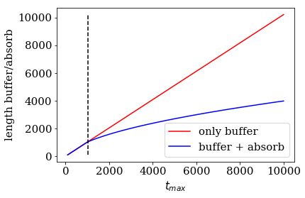
Comparison of the lead length for simple or absorbing boundary conditions

If the the maximal simulation time tmax is very small, we can always cut of all modes by a buffer zone that is large enough to cut off the fastest mode of the spectrum. We will therefore always find a trade off between required reflection refl_max and tmax.

Let us plot the total length of the lead cells, that is the sum of num_absorb_cells and buffer_cells, for different maximal simulation times tmax, keeping refl_max fixed. Note that our parameter estimate algorithm _monomial_parameter_estimate will use a sole buffer zone as a fallback in the case that the absorbing boundary conditions turn out to be disadvantageous. For for maximal simulation times on the left hand side of the black dashed line, simple boundary conditions perform better then absorbing boundary conditions, and vice versa for maximal simulation times choosen on the right-hand side of the back line. The automatic_boundary routine will therefore switch from SimpleBoundary to MonomialAbsorbingBoundary if tmax increses for refl_max.

def len_lead(tmax):
    tmp = tkwant.leads._monomial_parameter_estimate(spectrum, tmax, refl_max=1E-5,
                                                    degree=6, emax=fermi_energy)
    num_absorb_cells, _, num_buffer_cells, *_ = tmp
    return num_absorb_cells + num_buffer_cells

times = np.linspace(100, tmax, 100)
buffer_len = [vmax * t / 2 for t in times]
absorb_len = [len_lead(t) for t in times]

plt.plot(times, buffer_len, 'r', label='only buffer')
plt.plot(times, absorb_len, 'b', label='buffer + absorb')
plt.plot([1037] * 2, [np.min(buffer_len), np.max(buffer_len)], 'k--')
plt.xlabel(r'$t_{max}$')
plt.ylabel(r'length buffer/absorb')
plt.legend()
plt.show()

2.12.6. References

[1] J. Weston and X. Waintal, Linear-scaling source-sink algorithm for simulating time-resolved quantum transport and superconductivity, Phys. Rev. B 93, 134506 (2016). [arXiv]