Alternative boundary conditions¶

The physical system in this example is similar to Evolution of a scattering state under a voltage pulse in a quantum dot.

tkwant features highlighted

Selecting boundary conditions manually
Impact of the boundary type on performance

import time as timer
import numpy as np
from matplotlib import pyplot as plt

import kwant
import tkwant


def make_system(a=1, gamma=1.0, radius=10):
    """Make a tight binding system on a single square lattice"""
    # `a` is the lattice constant and `gamma` the hopping integral
    # both set by default to 1 for simplicity.

    lat = kwant.lattice.square(a, norbs=1)

    syst = kwant.Builder()

    # Define the quantum dot
    def circle(pos):
        (x, y) = pos
        return x ** 2 + y ** 2 < radius ** 2

    syst[lat.shape(circle, (0, 0))] = 4 * gamma
    syst[lat.neighbors()] = -gamma

    lead = kwant.Builder(kwant.TranslationalSymmetry((-1, 0)))
    lead[(lat(0, j) for j in range(-radius // 2 + 2, radius // 2 - 1))] = 4 * gamma
    lead[lat.neighbors()] = -gamma

    syst.attach_lead(lead)
    syst.attach_lead(lead.reversed())

    return syst


# for adding a time-dependent voltage on top of the leads
def faraday_flux(time):
    return 0.05 * (time - 10 * np.sin(0.1 * time))


def evolve(times, psi, operator):
    ops = []
    for time in times:
        psi.evolve(time)
        expectation = psi.evaluate(operator)
        ops.append(expectation)
    return ops


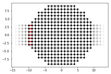
def main():
    syst = make_system()

    # add a time-dependent voltage to lead 0 -- this is implemented
    # by adding sites to the system at the interface with the lead and
    # multiplying the hoppings to these sites by exp(-1j * faraday_flux(time))
    extra_sites = tkwant.leads.add_voltage(syst, 0, faraday_flux)
    lead_syst_hoppings = [(s, site) for site in extra_sites
                          for s in syst.neighbors(site)
                          if s not in extra_sites]

    kwant.plot(syst, site_color='k', lead_color='grey', num_lead_cells=4,
               hop_lw=lambda a, b: 0.3 if (a, b) in lead_syst_hoppings else 0.1,
               hop_color=lambda a, b: 'r' if (a, b) in lead_syst_hoppings else 'k')

    syst = syst.finalized()

    # create an observable for calculating the current flowing from the left lead
    current_operator = kwant.operator.Current(syst, where=lead_syst_hoppings,
                                              sum=True)

    energy = 1.
    tmax = 600

    # create initial scattering state
    scattering_states = kwant.wave_function(syst, energy=energy, params={'time': 0})
    psi_st = scattering_states(0)[0]

    # maximal velocity of a mode in the leads
    vmax = 2 * np.linalg.norm(syst.leads[0].inter_cell_hopping(), ord=2)
    num_buffer_cells = int(vmax * tmax / 2)

    # boundary conditions typically used by `tkwant.solve`
    simple_boundaries = [tkwant.leads.SimpleBoundary(num_buffer_cells)
                         for l in syst.leads]

    # boundary conditions with an absorbing potential that increases
    # according to x**n where `x` is the distance into the lead
    absorbing_boundaries = [tkwant.leads.MonomialAbsorbingBoundary(num_absorb_cells=100,
                                                                   strength=10,
                                                                   degree=6)
                            for l in syst.leads]

    # create time-dependent wavefunctions that starts in a scattering state
    # originating from the left lead, using two different types of boundary
    # conditions
    psi_simple = tkwant.onebody.WaveFunction.from_kwant(syst=syst, psi_init=psi_st,
                                                        boundaries=simple_boundaries,
                                                        energy=energy)

    psi_alt = tkwant.onebody.WaveFunction.from_kwant(syst=syst, psi_init=psi_st,
                                                     boundaries=absorbing_boundaries,
                                                     energy=energy)

    # evolve forward in time, calculating the current
    times = np.arange(0, tmax)

    # Simple boundary conditions
    start = timer.process_time()
    current_simple = evolve(times, psi_simple, current_operator)
    stop = timer.process_time()
    print('Simple Boundary conditions elapsed time: {:.2f}s'.format(stop - start))

    # Absorbing boundary conditions
    start = timer.process_time()
    current_alt = evolve(times, psi_alt, current_operator)
    stop = timer.process_time()
    print('Absorbing Boundary conditions elapsed time: {:.2f}s'.format(stop - start))

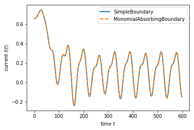
    plt.plot(times, current_simple, lw=2, label='SimpleBoundary')
    plt.plot(times, current_alt, '--', lw=2, label='MonomialAbsorbingBoundary')
    plt.xlabel(r'time $t$')
    plt.ylabel(r'current $I(t)$')
    plt.legend()
    plt.show()


if __name__ == '__main__':
    main()

../_images/alternative_boundary_conditions_1_1.png

Simple Boundary conditions elapsed time: 7.69s

Absorbing Boundary conditions elapsed time: 4.50s

../_images/alternative_boundary_conditions_1_4.png