Comparision between bias chemical potential and bias electrical potential
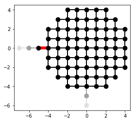
We consider a circular shaped central scattering region with two leads attached on the left and on the lower site as shown below. The left lead has an additional bias potential \(V_b\). In second quantization, the Hamiltonian is
where \(\gamma_{ii} = 4\) and for nearest-neighbors \(\gamma_{ij} = -1\). We are interested in the time-dependent current \(I(t)\) through the coupling element (highlighted in red in the system plot) from the left lead to the central scattering region:
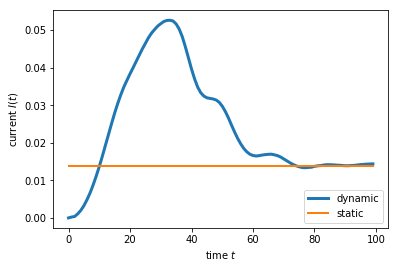
Two different results are obtained whether the potential \(V_b\) is explicitly time dependent or not. We refer to Ref. 1 for more information.
Static voltage
In the static case, the potential has a constant value \(V_b \equiv V = 0.5\). One can calculate the constant value of the current directly from the solution of above equations at the initial time \(t = 0\).
Dynamic voltage pulse
In the dynamic case the potential is zero at the initial time, but is switched on smoothly to reach the similar value as in the static case. We parametrize the potential as
such that the phase is
Performing a gauge transform, the time-dependent lead potential can be absorbed in the time-dependent system-lead coupling element between \(i_b\) and \(i_b + 1\):
The result obtained from the static and from the dynamic case are shown below.
tkwant features highlighted
Use of
tkwant.manybody.Stateto solve the manybody Schrödinger equation.Use of
refine_intervalsfor adaptive refinement the manybody integral.Use of
tkwant.leads.add_voltageto add time-dependence to leads.
import tkwant
import kwant
from math import sin, pi
import matplotlib.pyplot as plt


def am_master():
    """Return true for the MPI master rank"""
    return tkwant.mpi.get_communicator().rank == 0


def plot_currents(times, dynamic_current, static_current):
    plt.plot(times, dynamic_current, lw=3, label='dynamic')
    plt.plot([times[0], times[-1]], [static_current] * 2, lw=2, label='static')
    plt.legend(loc=4)
    plt.xlabel(r'time $t$')
    plt.ylabel(r'current $I(t)$')
    plt.show()


def circle(pos):
    (x, y) = pos
    return x ** 2 + y ** 2 < 5 ** 2


def make_system():
    gamma = 1
    lat = kwant.lattice.square(norbs=1)
    syst = kwant.Builder()
    syst[lat.shape(circle, (0, 0))] = 4 * gamma
    syst[lat.neighbors()] = -1 * gamma

    def voltage(site, V_static):
        return 2 * gamma + V_static

    lead = kwant.Builder(kwant.TranslationalSymmetry((-1, 0)))
    lead[lat(0, 0)] = voltage
    lead[lat.neighbors()] = -1 * gamma

    leadr = kwant.Builder(kwant.TranslationalSymmetry((0, -1)))
    leadr[lat(0, 0)] = 2 * gamma
    leadr[lat.neighbors()] = -1 * gamma

    syst.attach_lead(lead)
    syst.attach_lead(leadr)
    return lat, syst


def faraday_flux(time, V_dynamic):
    omega = 0.1
    t_upper = pi / omega
    if 0 <= time < t_upper:
        return V_dynamic * (time - sin(omega * time) / omega) / 2
    return V_dynamic * (time - t_upper / 2)


def tkwant_calculation(syst, operator, tmax, chemical_potential, V_static, V_dynamic):

    params = {'V_static': V_static, 'V_dynamic': V_dynamic}

    # occupation -- for each lead
    occup_left = tkwant.manybody.lead_occupation(chemical_potential + V_static)
    occup_lower = tkwant.manybody.lead_occupation(chemical_potential)
    occupations = [occup_left, occup_lower]

    # Initialize the time-dependent manybody state. Here we use a lower
    # accuracy for the initial adaptive refinement (at time=0) to speed up the calculation.
    # For a realistic simulation, set rtol and atol to smaller values.
    state = tkwant.manybody.State(syst, tmax, occupations, params=params, refine=False)
    state.refine_intervals(rtol=0.05, atol=0.05)

    # loop over time, calculating the current as we go
    expectation_values = []
    times = range(tmax)
    for time in times:
        state.evolve(time)
        # For a realistic simulation, one must set rtol and atol to smaller values,
        # or remove both arguments completely, to converge the manybody integral.
        state.refine_intervals(rtol=0.05, atol=0.05)
        result = state.evaluate(operator)
        expectation_values.append(result)
    return times, expectation_values


def main():

    lat, syst = make_system()

    # add the "dynamic" part of the voltage
    added_sites = tkwant.leads.add_voltage(syst, 0, faraday_flux)
    left_lead_interface = [(a, b)
                           for b in added_sites
                           for a in syst.neighbors(b) if a not in added_sites]
    if am_master():
        kwant.plot(syst, site_color='k', lead_color='grey',
                   hop_lw=lambda a, b: 0.3 if (a, b) in left_lead_interface else 0.1,
                   hop_color=lambda a, b: 'red' if (a, b) in left_lead_interface else 'k')

    syst = syst.finalized()

    # observables
    current_operator = kwant.operator.Current(syst, where=left_lead_interface)

    chemical_potential = 1
    tmax = 100

    # all the voltage applied via the time-dependenece
    V_static = 0
    V_dynamic = 0.5
    times, dynamic_current = tkwant_calculation(syst, current_operator, tmax,
                                                chemical_potential,
                                                V_static, V_dynamic)

    # all the voltage applied statically
    # even though we are doing a "tkwant calculation", we only calculate
    # the results at t=0.
    V_static = 0.5
    V_dynamic = 0
    _, (static_current, *_) = tkwant_calculation(syst, current_operator, 1,
                                                 chemical_potential,
                                                 V_static, V_dynamic)

    if am_master():
        plot_currents(times, dynamic_current, static_current)


if __name__ == '__main__':
    main()
See also
The complete source code of this example can be found in
voltage_raise.py.
References
- 1
B. Gaury, J. Weston, M. Santin, M. Houzet, C. Groth and X. Waintal, Numerical simulations of time-resolved quantum electronics, Phys. Rep. 534, 1 (2014). [arXiv]