Evolution of a scattering state under a voltage pulse in a quantum dot
Problem formulation
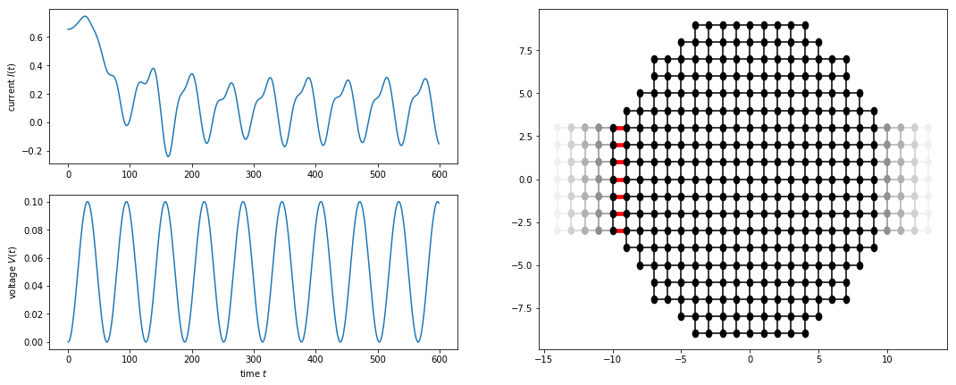
We consider a circular shaped central scattering region with two leads attached on the left and on the right-hand side as shown below. The system is perturbed by a time-dependent voltage pulse \(V_p(t)\) which is injected into the left lead. We evolve a single onebody scattering states of the system forward in time and calculate the expectation value of the current.
Explicitly, the Hamiltonian is
The second term of \(\hat{H}(t)\) accounts for the time-dependent voltage pulse
such that the phase is
The time-dependent couplings between the system and the left lead (between the lattice positions \(i_p = -10\) and \(i_p + 1 = -9\)), are highlighed in red in the figure below.
The current in positive x direction through a system-lead coupling element is
where \(\alpha \equiv (i_p, y)\) and \(\beta \equiv (i_p+1, y)\) label the grid position in x and y direction. Summing in y direction, we plot the total current through the system-lead interface
tkwant features highlighted
Use of
tkwant.leads.add_voltageto add time-dependence to leads.Use of
tkwant.onebody.ScatteringStatesto solve the time-dependent Schrödinger equation for an open system with an initial scattering state.
import numpy as np
import matplotlib
from matplotlib import pyplot as plt

import kwant
import tkwant


def make_system(a=1, gamma=1.0, radius=10, width=7):
    """Make a tight binding system on a single square lattice"""
    # `a` is the lattice constant and `gamma` the hopping integral
    # both set by default to 1 for simplicity.

    lat = kwant.lattice.square(a, norbs=1)
    syst = kwant.Builder()

    # Define the quantum dot
    def circle(pos):
        (x, y) = pos
        return x ** 2 + y ** 2 < radius ** 2

    syst[lat.shape(circle, (0, 0))] = 4 * gamma
    syst[lat.neighbors()] = -gamma

    lead = kwant.Builder(kwant.TranslationalSymmetry((-1, 0)))
    lead[(lat(0, j) for j in range(-(width - 1) // 2, width // 2 + 1))] = 4 * gamma
    lead[lat.neighbors()] = -gamma
    syst.attach_lead(lead)
    syst.attach_lead(lead.reversed())

    return syst


def faraday_flux(time):
    return 0.05 * (time - 10 * np.sin(0.1 * time))


def main():

    # create a system andadd a time-dependent voltage to lead 0 -- this is
    # implemented by adding sites to the system at the interface with the lead
    # and multiplying the hoppings to these sites by exp(-1j * faraday_flux(time))
    syst = make_system()

    added_sites = tkwant.leads.add_voltage(syst, 0, faraday_flux)
    interface_hoppings = [(a, b)
                          for b in added_sites
                          for a in syst.neighbors(b) if a not in added_sites]

    fsyst = syst.finalized()

    current_operator = kwant.operator.Current(fsyst, where=interface_hoppings,
                                              sum=True)

    times = np.arange(0, 600)

    # create a time-dependent wavefunction that starts in a scattering state
    # originating from the left lead
    mode = 0
    psi = tkwant.onebody.ScatteringStates(fsyst, energy=1., lead=0,
                                          tmax=max(times))[mode]

    # evolve forward in time, calculating the current
    current = []
    for time in times:
        psi.evolve(time)
        current.append(psi.evaluate(current_operator))

    # plot results
    plt.figure(figsize=(18, 7))

    gs = matplotlib.gridspec.GridSpec(2, 2)

    ax1 = plt.subplot(gs[0, 0])
    ax1.plot(times, current)
    ax1.set_ylabel(r'current $I(t)$')

    ax2 = plt.subplot(gs[1, 0])
    ax2.plot(times, 0.05 * (1 - np.cos(0.1 * times)))
    ax2.set_xlabel(r'time $t$')
    ax2.set_ylabel(r'voltage $V(t)$')

    ax3 = plt.subplot(gs[:, 1])
    kwant.plot(syst, ax=ax3, site_color='k', lead_color='grey', num_lead_cells=4,
               hop_lw=lambda a, b: 0.3 if (a, b) in interface_hoppings else 0.1,
               hop_color=lambda a, b: 'r' if (a, b) in interface_hoppings else 'k')
    plt.show()

if __name__ == '__main__':
    main()
See also
The complete source code of this example can be found in
open_system.py.