Pulse propagation in a graphene quantum dot
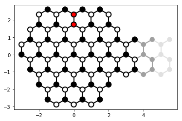
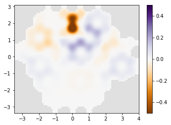
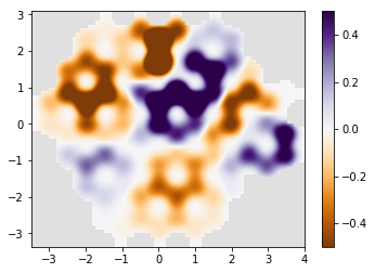
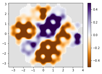
The physical system in this example is a downscaled version of the “graphene quantum billard” from Ref. [1]. An irregular shaped graphene dot, which is subjected to a time-dependent perturbation (the two red sites of the system plot are perturbed by a Gaussian shaped pulse). We calculate several snapshots of the electron density after the perturbation has been applied. While the accuracy and parameters are arbitrary and tuned to speed up the calculation, this example shows that graphene can be studied in a similar way.
import tkwant
import kwant
import numpy as np
import matplotlib.pyplot as plt
import functools as ft


def am_master():
    """Return true for the MPI master rank"""
    return tkwant.mpi.get_communicator().rank == 0


def side_color_func(site):
    return 'r' if electrode_shape(site.pos) else ('k' if site.family == a else 'w')


def onsite_potential(site, time):
    # Time-dependent potential (static part + V(t))
    return 0.001 * np.exp(- 0.01 * (time - 20)**2)


def circle(pos, x0, y0, r):
    x, y = pos
    return (x - x0)**2 + (y - y0)**2 < r**2


def electrode_shape(pos):
    x, y = pos
    return (-0.1 < x < 0.1) and (1 < y < 3)


def lead_shape(site):
    x, y = site.pos
    return (-1.5 < y < 1.0)


def make_system():
    # Define the graphene lattice.
    lat = kwant.lattice.honeycomb(a=1, norbs=1)
    a, b = lat.sublattices

    # Create graphene model.
    model = kwant.Builder(kwant.TranslationalSymmetry(
        lat.vec((1, 0)), lat.vec((0, 1))))
    model[[a(0, 0), b(0, 0)]] = 0
    model[lat.neighbors()] = -1

    # Central scattering region.
    funs = [ft.partial(circle, x0=0, y0=0, r=3.3)]
    syst = kwant.Builder()
    syst.fill(model, lambda site: any(f(site.pos) for f in funs), a(0, 0))
    syst.eradicate_dangling()
    syst[lat.shape(electrode_shape, (0, 2))] = onsite_potential

    # Define the lead using a trick to avoid ugly diagonal lead interfaces.
    sym = kwant.TranslationalSymmetry(lat.vec((1, 0)))
    sym.add_site_family(a, other_vectors=[(-1, 2)])
    sym.add_site_family(b, other_vectors=[(-1, 2)])

    lead = kwant.Builder(sym)
    lead.fill(model, lead_shape, a(0, 0))
    syst.attach_lead(lead)

    return syst


chemical_potential = -2.5
times = [10, 15, 20, 25, 30]

syst = make_system()

# plot the system
lat = kwant.lattice.honeycomb(a=1, norbs=1)
a, b = lat.sublattices
if am_master():
    kwant.plot(syst, site_lw=0.1, site_color=side_color_func,
               lead_site_lw=0, lead_color='grey')

syst = syst.finalized()

density_operator = kwant.operator.Density(syst)
occupations = tkwant.manybody.lead_occupation(chemical_potential)

# Initialize the time-dependent manybody state. Here we use a lower
# accuracy for the initial adaptive refinement (at time=0) to speed up the calculation.
# For a realistic simulation, set rtol and atol to smaller values.
state = tkwant.manybody.State(syst, max(times), occupations, refine=False)
state.refine_intervals(rtol=1.5E-2, atol=1.5E-2)


# simulation
density0 = state.evaluate(density_operator)
densities = []
for time in times:
    state.evolve(time)
    # For a realistic simulation, one must set rtol and atol to smaller values,
    # or remove both arguments completely, to converge the manybody integral.
    state.refine_intervals(rtol=0.1, atol=0.1)
    density = state.evaluate(density_operator)
    if am_master():
        densities.append(density - density0)

# plot the result
if am_master():
    normalization = 1 / np.max(densities)
    for time, density in zip(times, densities):
        density *= normalization
        print('time={}'.format(time))
        kwant.plotter.density(syst, density, relwidth=0.15,
                              cmap='PuOr', vmin=-0.5, vmax=0.5)
time=10
time=15
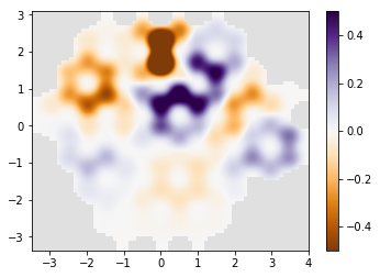
time=20
time=25
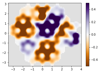
time=30
See also
The complete source code of this example can be found in
graphene.py.
References
[1] T. Kloss, J. Weston, B. Gaury, B. Rossignol, C. Groth and X. Waintal, Tkwant: a software package for time-dependent quantum transport New J. Phys. 23, 023025 (2021), arXiv:2009.03132 [cond-mat.mes-hall].