The simplest Tkwant problem: DC current through a 1D chain¶

Note

Also in this tutorial: two different ways of applying a bias voltage, electrical potential drop versus chemical potential drops

In this tutorial, we use Tkwant to revisit a simple problem that actually does not require time-dependent simulations: the DC current-voltage \(I(V)\) characteristics of a perfectly transmitting one-dimensional chain. This benchmark example allows us to check that Tkwant is capable of recovering the stationary limit at long time. It also illustrates most Tkwant features in a minimum setup, hence can be used as a first exposition to Tkwant. More importantly, it allows one to understand the practical difference between a drop of chemical potential and a drop of electric potential and show that the two concepts are not (always) interchangeable.

Previous discussion of this problem can be found in section 8.4 of Ref. [1].

Problem definition¶

We consider electron transport on a infinitly long one-dimensional wire described by a nearest neighbour tight-binding model.

\[\begin{align} H &= -\gamma \sum_{i=-\infty}^\infty c^\dagger_{i+1} c_{i} + \text{h.c.} \tag{1} \end{align}\]

where \(c^\dagger_i\) (\(c_i\)) are the fermionic creation (annihilation) operator on site \(i\) and \(\gamma\) is the hopping matrix element. The dispersion relation of the electrodes is simply given by \(E(k) = - 2 \gamma \cos(k)\). The left lead (\(i\le 0\)) is described by a Fermi function \(f_L\) with chemical potential \(\mu_L\) and the right lead (\(i>0\)) by \(\mu_R\). We focus on the zero temperature case so that \(f_L(E)= \Theta(\mu_L-E)\) and \(f_R(E)= \Theta(\mu_R-E)\).

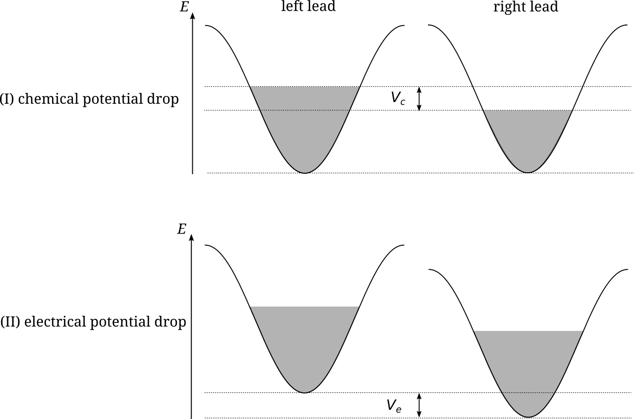
We apply a difference of potential \(V\) between the two electrodes. We consider two different situations that lead to two different steady-state current flow through the wire, see Fig. 1.

1. drop of chemical potential: \(V=\mu_L-\mu_R\). The filling of the bands of the two electrodes is different, while the energy position of the bottom of the two bands is the same.
1. drop of eletrical potential: \(\mu_L=\mu_R\), the filling of both bands is the same, but the bottom of the band of the left electrode is shifted by \(V\) with respect to the bottom of the band of the right electrode.

In the following, we will show two concurring methods to calculate the current for each of the two cases. In general the drop of potential is a linear combination of case I and II and a self-consistent quantum-electrostatic problem must be solved to find the correct boundary condition, see the corresponding discussion in Ref. [1].

Different approaches (Theory)¶

(I) Chemical potential drop¶

The chemical potential drop is the usual situation considered in the Landauer-Buttiker formalism. Applying the drop simply amounts to shifting one chemical potential by \(V\) with respect to the other one: \(\mu_L = \mu + V\) and \(\mu_R = \mu\).

Method A: Using the scattering matrix¶

In the scattering matrix approach, the current can be obtained from the Landauer formula,

\[\begin{align} I(V) &= \int_{\mu}^{\mu + V} d E \, T(E) \tag{2} \end{align}\]

where \(T(E)\) is the transmission. As the system described by Eq. (1) has no reflection, \(T(E)=1\) inside the band and zero outside, i.e. For \(\mu = 0\), the transmission is \(T(E) = \Theta(2 - E) \Theta(2 + E)\), such that the current (in units of \(e \gamma / h\)) is

\[\begin{split}\begin{align} I(V) &= \begin{cases} V & \text{if } |V| < 2 \\ 2 \text{sgn}(V) & \text{if } |V| \geq 2 \end{cases} \tag{3} \end{align}\end{split}\]

Method B: Using the scattering wave function¶

In the wave function approach, the current from site \(b\) to site \(a\) (in units of \(e \gamma / \hbar\)) can be calculated from

\[\begin{equation} I_{ab}(t) = - 2 i \textrm{Im} \int \frac{d E}{2 \pi} \sum_{\alpha} f_\alpha(E) \psi_{\alpha E}^*(t, a) H_{ab} \psi_{\alpha E}(t, b). \tag{4} \end{equation}\]

where \(\psi_{\alpha E}(t, i)\) is the scattering wave function for lead \(\alpha\), site index \(i\) and time \(t\), and \(f_\alpha\) is the Fermi function. As before we consider non-interacting electrons at zero temperature, such that \(f_\alpha(E) = \Theta(\mu_\alpha - E)\).

Since this problem does not depend on time, we can caclculate the current at any time and get the same result, i.e. we can fix \(t = 0\). Also, in the steady-state current conservation implies that the current does not depend on space neither, i.e. we can fix \(a = 1\) and \(b = 0\):

\[\begin{equation} I = 2 \pi I_{1, 0}(t=0) \tag{5} \end{equation}\]

Note the factor \(2 \pi\) needed to convert to the same units of \(e \gamma / h\) as Eq. (2).

(II) Electrical potential drop¶

To apply a drop of electric potential, we need to modify the Hamiltonian and shift the electric potential of the left lead by \(V\),

\[\begin{align} H &= -\gamma \sum_{i=-\infty}^\infty c^\dagger_{i+1} c_{i} + \text{h.c.} + V \sum_{i=-\infty}^0 c^\dagger_{i} c_{i} \tag{6} \end{align}\]

We also shift the chemical potential accordingly as \(\mu_L = \mu + V, \, \mu_R = \mu\) to have identical fillings of both leads.

Method A: Using the scattering matrix¶

In the scattering matrix approach, the current can be calculated using Landauer formula, same as Eq. (2), as

\[\begin{align} I(V) &= \int_{\mu}^{\mu + V} d E \, T_{V}(E) \tag{7}. \end{align}\]

However, the drop of electrical potential now implies some reflection so that the transmission probability is perfect anymore. Also for large bias, the misalignement between the bands imply that the current must vanish in sharp contrast to the chemical potential drop situation. Below, we perform the calculation of \(T_{V}(E)\) numerically with Kwant as it is rendered non-trivial by the potential drop.

Method B and C: Wave function approach - steady-state and transient regime¶

As in case I, the steady-state current could also be obtained by the wave fuction approach using Eqs. (4) and (5) (method B). To make the problem time-dependent, we consider another situation (method C) where the system is initially at equilibrium with \(V=0\) and at \(t=0\), we switch on the electric potential drop. In other words, we make Eq. (6) time dependent, by replacing \(V \rightarrow V(t)\). The function \(V(t)\) can be arbitrary as long as \(V(t=0) = 0\) and \(V(t)=V\) for a large enough time. We will study the corresponding trnasient problem with Tkwant.

Using the gauge transformation

\[\begin{align} U(t) &= e^{- i \phi(t) \sum_{i=-\infty}^0 c^\dagger_{i} c_{i}}, \quad \phi(t) = \int_{-\infty}^t V (t') dt' \end{align}\]

the Hamiltonian transforms to

\[\begin{split}\begin{align} \bar{H} &= U H U^\dagger - i U \frac{\partial}{\partial t} U^\dagger = \nonumber \\ &= -\gamma \sum_{i=-\infty}^\infty c^\dagger_{i+1} c_{i} - \gamma [e^{- i \phi(t)} - 1] c^\dagger_{1} c_{0} + \text{h.c.} \tag{8} \end{align}\end{split}\]

We see that the left part of the system is again time independent, but that only the hopping element \(\gamma c^\dagger_1 c_0\) at the potential drop in Hamiltonian Eq. (6), (and its hermitian conjugate), has aquired a time dependent phase \(e^{- i \phi(t)} \gamma c^\dagger_1c _0\). Here we make the simple choice of a sharp quench \(V(t) = V \Theta(t)\) to switch on the potential at the initial time \(t = 0\), such that

\[\begin{align} \phi(t) = V t \tag{9} \end{align}\]

Suppose that we are able to calculate the time-dependent scattering states with Hamiltonian Eq. (8), the non-steady state current can be obtained again with Eq. (4). Using the convention

\[\begin{equation} I(t) = 2 \pi I_{1, 0}(t) \tag{10} \end{equation}\]

one should find that the result of Eq.(10) converges to the same result as Eq. (7) for time \(t\) large enough for the system to reach the steady-state.

The two different \(I(V)\) characteristics¶

The \(I(V)\) characteristics for the two different cases I and II is shown below in figure 2. It can also be found in figure 9 in Ref. [1]: For small values of the potential \(V\), the steady-state current depends linearly on \(V\) and is essentially identical in both cases. Only for large values of \(V\), the current will reach a plateau for case (I), whereas it goes down to zero in case (II).

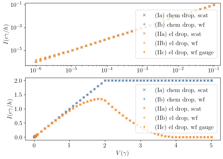
Note that the different methods for each case agree pretty accurately, except for the small missmatch in case (II) at very small \(V \sim 10^{-6}\). Increasing the numerical accuracy (by adjusting \(\texttt{atol}\) and \(\texttt{rtol}\) in \(\texttt{refine_intervals()}\)), this mismatch can be removed as well.

Different approaches (Numerical Solutions)¶

To calculate the current in practice, we need to compute the scattering matrix and the (time-dependent) wave function. We will show how to do this using the Python packages Kwant [2] and Tkwant [3].

We first include standard Python packages alongside Kwant, Tkwant and KwantSpectrum [3].

import tkwant
import kwant
import kwantspectrum as ks
import numpy as np
import scipy
import cmath
import matplotlib.pyplot as plt

(I) Chemical potential drop¶

The Hamiltonian Eq. (1) can be modeled with Kwant as

def make_system(a=1):

    lat = kwant.lattice.square(a=a, norbs=1)
    syst = kwant.Builder()

    # central system
    syst[(lat(i, 0) for i in [0, 1])] = 0
    syst[lat.neighbors()] = -1

    # leads
    lead = kwant.Builder(kwant.TranslationalSymmetry((-a, 0)))
    lead[lat(0, 0)] = 0
    lead[lat.neighbors()] = -1
    syst.attach_lead(lead)
    syst.attach_lead(lead.reversed())

    return syst, lat

syst, lat = make_system()
syst = syst.finalized()

The parameters \(\mu\) and \(V\) are set to:

mu = 0
v = 0.1

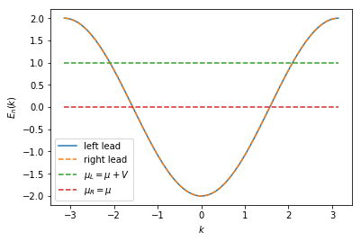
The spectrum for the left and the right lead is similar, only the chemical potential, which sets the filling, is different. For illustrative reasons, we plot the spectrum and the chemical potentials with a 10 times larger value for \(V\) to better see the different fillings by eye.

momenta = np.linspace(-np.pi, np.pi, 500)
specs = ks.spectra(syst.leads)
plt.plot(momenta, specs[0](momenta, 0), label=r'left lead')
plt.plot(momenta, specs[1](momenta, 0), '--', label=r'right lead')
plt.plot([-np.pi, np.pi], 2 * [mu + 10 * v], '--', label=r'$\mu_L = \mu + V$')
plt.plot([-np.pi, np.pi], 2 * [mu], '--', label=r'$\mu_R = \mu$')
plt.xlabel(r'$k$')
plt.ylabel(r'$E_{n}(k)$')
plt.legend()
plt.show()

A: Steady-state current from the scattering matrix using Kwant¶

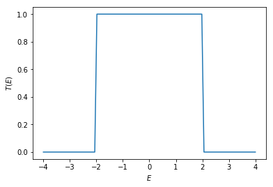
The transmission \(T\) can be calculated using \(\texttt{kwant.smatrix.transmission()}\). As a function of energy \(E\), the transmission is equal one within the band opening and zero otherwise.

def transmission(energy):
    try:
        smatrix = kwant.smatrix(syst, energy=energy)
        res = smatrix.transmission(1, 0)
    except:  # exactly at the band opening, the kwant smatrix crashes
        res = 0
    return res

energies = np.linspace(-4, 4, 100)
trans = [transmission(en) for en in energies]

plt.plot(energies, trans)
plt.xlabel(r'$E$')
plt.ylabel(r'$T(E)$')
plt.show()

The current follows from Eq. (2) and (3) as

def current_v(v):
    return min(2, v)

print('current={:10.4e}'.format(current_v(v)))  # units (e \gamma / h)

current=1.0000e-01

Steady-state current from the wave function approach using Tkwant¶

We first set the chemical potential for the left (\(\mu_L = \mu + V\)) and right lead (\(\mu_R = \mu\)). We also define the (Kwant) operator to measure the current flowing trough the central system from left to right.

# occupation of left and right lead
occupations = [tkwant.manybody.lead_occupation(chemical_potential=mu+v),
               tkwant.manybody.lead_occupation(chemical_potential=mu)]

# current from site 0 to site 1
current_operator = kwant.operator.Current(syst, where=[(lat(1, 0), lat(0, 0))])

The next two lines evaluate the current equation (4) and (5) at initial time \(t = 0\). One still needs to provide an upper time, but its actual value is irrelevant for the result and is required only to be larger than zero.

state = tkwant.manybody.State(syst, tmax=1, occupations=occupations)
current = state.evaluate(current_operator)

print('current= {:10.4e}'.format(2 * np.pi * current))  # units (e \gamma / h)

current= 1.0000e-01

(II) Electrical potential drop¶

The Hamiltonian Eq. (6) can be modeled with Kwant as

def make_system(a=1):

    def onsite(site, v):
        return v

    # central system
    lat = kwant.lattice.square(a=a, norbs=1)
    syst = kwant.Builder()

    syst[(lat(i, 0) for i in [0, 1])] = 0
    syst[lat.neighbors()] = -1

    # leads
    lead_left = kwant.Builder(kwant.TranslationalSymmetry((-a, 0)))

    lead_left[lat(0, 0)] = onsite
    lead_left[lat.neighbors()] = -1
    syst.attach_lead(lead_left)

    lead_right = kwant.Builder(kwant.TranslationalSymmetry((-a, 0)))

    lead_right[lat(0, 0)] = 0
    lead_right[lat.neighbors()] = -1

    syst.attach_lead(lead_right.reversed())

    return syst, lat

syst, lat = make_system()
syst = syst.finalized()

The parameters for \(\mu\) and \(V\) are set to:

mu = 0
v = 0.1

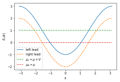
The energy dispersion for the left and the right lead is now different and shifted by \(V\). The chemical potential has to be shifted by the same value in order to lead to half filling for each lead. For illustrative reasons, we plot the spectrum with a 10 times larger value for \(V\) to better see the different fillings by eye.

momenta = np.linspace(-np.pi, np.pi, 500)
specs = ks.spectra(syst.leads, params={'v': 10 * v})
plt.plot(momenta, specs[0](momenta, 0), label=r'left lead')
plt.plot(momenta, specs[1](momenta, 0), '--', label=r'right lead')
plt.plot([-np.pi, np.pi], [mu + 10 * v, mu + 10 * v], '--', label=r'$\mu_L = \mu + V$')
plt.plot([-np.pi, np.pi], [mu, mu], '--', label=r'$\mu_R = \mu$')
plt.xlabel(r'$k$')
plt.ylabel(r'$E_{n}(k)$')
plt.legend()
plt.show()

Steady-state current from the scattering matrix using Kwant¶

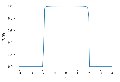
The transmission coefficient \(T_{V}\) can be calculated again with \(\texttt{kwant.smatrix.transmission()}\). For \(V \neq 0\), the transmission coefficient is a nonlinear function of the energy \(E\).

def transmission(energy, v):
    try:
        smatrix = kwant.smatrix(syst, energy=energy, params={"v": v})
        res = smatrix.transmission(1, 0)
    except:  # exactly at the band opening, the kwant smatrix crashes
        res = 0
    return res

energies = np.linspace(-4, 4, 100)
trans = [transmission(en, v) for en in energies]

plt.plot(energies, trans)
plt.xlabel(r'$E$')
plt.ylabel(r'$T_{V}(E)$')
plt.show()

The current follows from Eq. (7) as:

def current_v(v):
    def transfunc(energy):
        return transmission(energy, v)
    return scipy.integrate.quad(transfunc, 0, v)[0]

print('current={:10.4e}'.format(current_v(v)))  # units (e \gamma / h)

current=9.9937e-02

Steady-state current from the wave-function using Tkwant¶

We set the chemical potential for the left (\(\mu_L = \mu + V\)) and right lead (\(\mu_R = \mu\)). The (Kwant) operator measures the current flowing trough the central system from left to right.

# occupation of left and right lead
occupations = [tkwant.manybody.lead_occupation(chemical_potential=mu+v),
               tkwant.manybody.lead_occupation(chemical_potential=mu)]

# current from site 0 to site 1
current_operator = kwant.operator.Current(syst, where=[(lat(1, 0), lat(0, 0))])

Then current Eq. (4) and (5) is evaluated from manybody state at initial time \(t = 0\). One still needs to provide an upper time, but its actual value is irrelevant for the result and is required only to be larger than zero.

state = tkwant.manybody.State(syst, tmax=1, occupations=occupations, params={'v': v})
current_ss = state.evaluate(current_operator)

print('current= {:10.4e}'.format(2 * np.pi * current_ss))  # units (e \gamma / h)

current= 9.9938e-02

Transient current from the wave-function using Tkwant¶

The Hamiltonian Eq. (8) can be modeled with Kwant as

def coupling_nn(site1, site2, time, v):
    phi = v * time
    return - cmath.exp(- 1j * phi)


def make_system(a=1):

    lat = kwant.lattice.square(a=a, norbs=1)
    syst = kwant.Builder()

    syst[(lat(i, 0) for i in [-1, 0, 1])] = 0
    syst[lat.neighbors()] = -1

    # time dependent coupling - e^(-i \phi(t)) c^\dagger_0 c_{-1}
    syst[(lat(0, 0), lat(-1, 0))] = coupling_nn

    lead = kwant.Builder(kwant.TranslationalSymmetry((-a, 0)))
    lead[lat(0, 0)] = 0
    lead[lat.neighbors()] = -1
    syst.attach_lead(lead)
    syst.attach_lead(lead.reversed())

    return syst, lat

syst, lat = make_system()
syst = syst.finalized()

One needs to provide only one \(\texttt{tkwant.manybody.lead_occupation()}\) instance as the occupation in the left and in the right lead is similar. The (Kwant) operator measures the current flowing trough the central system from left to right.

# occupation of left and right lead
occupations = tkwant.manybody.lead_occupation(chemical_potential=mu)

# current from site 0 to site 1
current_operator = kwant.operator.Current(syst, where=[(lat(1, 0), lat(0, 0))])

The time evolution is then performed with the standard manybody state of Tkwant. One can simply pass \(V\) as an external parameter to the manybody state. We also need to refine the manybody integral along the evolution using \(\texttt{refine_intervals()}\) to obtain numerically accurate results.

times = np.linspace(0, 80, 501)

state = tkwant.manybody.State(syst, tmax=max(times), occupations=occupations, params={'v': v})

currents = []
for time in times:
    state.evolve(time)
    state.refine_intervals()
    current = state.evaluate(current_operator)
    currents.append(current)

currents = 2 * np.pi * np.array(currents)  # convert units to (e \gamma / h)

print('current= {:10.4e}'.format(currents[-1]))

current= 9.9947e-02

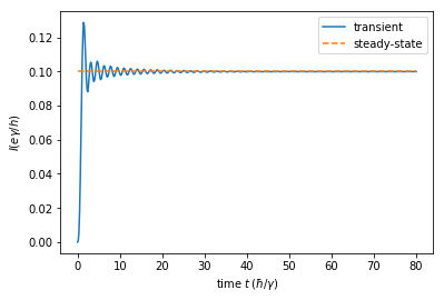
The current Eq. (10) is finally plotted as a function of time. It converges to the stationary value for large times, as expected.

plt.plot(times, currents, label="transient")
plt.plot([times[0], times[-1]], 2 * [2 * np.pi * current_ss], '--', label="steady-state")
plt.xlabel(r'time $t \, (\hbar / \gamma)$')
plt.ylabel(r'$I (e \gamma / h)$')
plt.legend()
plt.show()

References¶

[1] B. Gaury, J. Weston, M. Santin, M. Houzet, C. Groth, and X. Waintal, Numerical simulations of time-resolved quantum electronics Phys. Rep. 534, 1 (2014).

[2] C. W. Groth, M. Wimmer, A. R. Akhmerov, and X. Waintal, Kwant: a software package for quantum transport New J. Phys. 16, 063065 (2014).

[3] T. Kloss, J. Weston, B. Gaury, B. Rossignol, C. Groth and X. Waintal, Tkwant: a software package for time-dependent quantum transport New J. Phys. 23, 023025 (2021).

The simplest Tkwant problem: DC current through a 1D chain¶

Problem definition¶

Different approaches (Theory)¶

(I) Chemical potential drop¶

Method A: Using the scattering matrix¶

Method B: Using the scattering wave function¶

(II) Electrical potential drop¶

Method A: Using the scattering matrix¶

Method B and C: Wave function approach - steady-state and transient regime¶

The two different \(I(V)\) characteristics¶

Different approaches (Numerical Solutions)¶

(I) Chemical potential drop¶

A: Steady-state current from the scattering matrix using Kwant¶

Steady-state current from the wave function approach using Tkwant¶

(II) Electrical potential drop¶

Steady-state current from the scattering matrix using Kwant¶

Steady-state current from the wave-function using Tkwant¶

Transient current from the wave-function using Tkwant¶

References¶

Table of Contents

This Page