2.7. Green functions
2.7.1. Introduction
We consider a general quadratic Hamiltonian describing a noninteracting open tight-binding system
The \(c^\dagger_i,\, (c_i)\) are the usual Fermionic creation and annihilation operators of a one electron state at site \(i\), where the site index comprises all degreens of freedom of the system, such as lattice site, spin, orbital index etc. Moreover, an element of the Hamiltion matrix \(H_{ij}(t)\) can have an arbitrary time dependence. We are interested in the nonequilibrium Green function
where \(c^\dagger_i(t)\) and respectively \(c_i(t)\) correspond to the fermionic operators in the Heisenberg representation, the curly brackets \(\{ \ldots \}\) stand for the anticommutator and the manybody average \(\langle \ldots \rangle \equiv \textrm{Tr}(\hat{\rho} \ldots)\) where \(\hat{\rho}\) is the non-equilibrium density matrix at initial time. Note that above lesser and retarded Green functions are sufficient to obtain all other kind of Green functions [1] also in a general nonequilibrium situation, where no fluctucation-dissipation relation holds.
A numerically exact method to calculate \(G^<\) and \(G^R\) for quadratic Hamiltonians as Eq. (1) has been developed in [2] to express them in terms of the wave function $psi$ as
where \(f_\alpha\) is the Fermi function in lead \(\alpha\). This method has now been implemented in the Tkwant package [3]. After a short introduction to the corresponding Tkwant class we will show in this tutorial how different Green functions are calculated in practice using Tkwant. As a toy example we will use two impurity models on a one dimensional chain: (I) a double quantum dot in a stationary out-of-equilibrium regime and (II) a single impurity in the transient regime after a quench. Closed analytical expressions can be derived at weak coupling between the impurites and the semi-infinite leads in the so-called flatband approximation [4], which serve as a benchmark for the numerical Tkwant results. The detailled calculation of the analytical flat-band results are provided in the Appendix.
2.7.2. The class \(\texttt{tkwant.manybody.Greenfunction}\)
Tkwant provides the class \(\texttt{tkwant.manybody.Greenfunction}\) to compute nonequilibrium Greenfunctions between two sites of the central scattering system. The Green functions are real two-time objects which are also valid in the transient nonequilibrium regime. The class \(\texttt{tkwant.manybody.Greenfunction}\) is simple to use and behaves similar to the manybody wavefunction class \(\texttt{tkwant.manybody.State}\). The \(\texttt{tkwant.manybody.Greenfunction}\) class is instatiated as
green = tkwant.manybody.GreenFunction(syst, tmax, occupations)
where \(\texttt{syst}\) is a finalized Kwant system of type \(\texttt{kwant.builder.FiniteSystem}\), \(\texttt{tmax}\) is the maximal time such that \(t_0, t_1 \leq t_{max}\) for \(G(t_0, t_1)\) and occupations is a sequence of lead occupations of type \(\texttt{tkwant.manybody.Occupation}\). To calculate \(G^<_{i=0,j=2}(t_0, t_1)\) and \(G^>_{i=1, j=5}(t_0, t_1)\) for instance, both for time arguments \(t_0=8, t_1 =3\), one evaluates
green.evolve(time0=5, time1=3)
green.refine_intervals()
gless = green.lesser(i=0, j=2)
ggreat = green.greater(i=1, j=5)
The second call to the \(\texttt{refine_intervals()}\) method is optional, but is important to reach a numerically precise estimate of the manybody integral. Without further arguments, a default precision will be targeted for the diagonal Green function elements \(G_{ii}\) at the given times, where \(i\) runs over all sites of the central scattering region. One can change this behavior and pass a sequence of tuples \((i,j)\) to the \(\texttt{refine_intervals()}\) method, which will refine the corresponding \(G_{ij}\) elements in the sequence. For instance
green.refine_intervals(sites=[(0, 1), (2, 1)])
will refine the Green functions on sites \(G_{01}\) and \(G_{21}\). One can also change the relative and the absolute precision of the result via
green.refine_intervals(rtol=1e-8, atol=1e-8)
To obtain the other Green functions (retarded, keldysh, time-ordered…) is also possible as shown in section Various kinds of Green functions. We can now directly study the two toy problems.
2.7.3. Example I: A two sites impurity on an infinite one-dimensional chain (double quantum dot)
We depict two impurities on a one-dimensional chain described by the Hamiltonian
The sites \(i\) label the discrete lattice sites and the hoppings are \(\gamma_i = 1\) for all \(i\) except at the impurity, where we introduce the more descriptive notation \(\gamma_{-1} = \gamma_L\), \(\gamma_0 = \gamma_C\) and \(\gamma_1 = \gamma_R\). In both the left and the right lead far away from the central system, the electrons are considered to be in thermal equilibrium. For simplicity we choose the temperature to be zero in both leads, but allow two different chemical potentials \(\mu_L\) and \(\mu_R\) to realize a stationary non-equilibrium situation.
As the above problem is stationary in time, all Green functions depend only on the time difference
and we will plot effecitve single-time Green functions defined as
A true non-stationary problem, where translational time symmetry does not hold such that the Green functions have a true two-time dependence are consideren for model II below. The analytical calculation of the non-equilibrium Green functions in flatband approximation are given below. Let us state again that the wave function method in [2] which is implemented in Tkwant does not rely on the smallness of the coupling constants, but we choose this regime here in order to use the flatband limit as a benchmark.
Numerical calculation of \(G^<\) and \(G^R\) using Tkwant
We will show how to do this using the Python package Tkwant. First we include Tkwant [3] and Kwant [5] alongsinde standard Python packages.
import tkwant
import kwant

import numpy as np
import matplotlib.pyplot as plt
The parameters and timesteps are set to:
# couplings
gamma_L = 0.14
gamma_C = 0.05
gamma_R = 0.08

# onsite elements
epsilon_L = 0.5
epsilon_R = 0.3

# chemical potentials
mu_L = 0.5
mu_R = - 0.8

# values of time where the green’s function will be evaluated
times = np.linspace(0, 20, 21)
Building the Kwant system
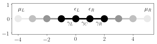
We build a standard one-dimensional Kwant system. The plot below visualizes again our model defind in Eq. (4).
def make_double_impurity_system(gamma_L, gamma_C, gamma_R, eps_L, eps_R):

    # system building
    lat = kwant.lattice.chain(a=1, norbs=1)
    syst = kwant.Builder()

    # central scattering region
    syst[(lat(x) for x in [-1, 2])] = 0
    syst[lat(0)] = eps_L
    syst[lat(1)] = eps_R

    syst[(lat(0), lat(-1))] = -gamma_L
    syst[(lat(1), lat(0))] = -gamma_C
    syst[(lat(2), lat(1))] = -gamma_R

    # add leads
    sym = kwant.TranslationalSymmetry((-1,))
    lead_left = kwant.Builder(sym)
    lead_left[lat(0)] = 0
    lead_left[lat.neighbors()] = -1
    syst.attach_lead(lead_left)
    syst.attach_lead(lead_left.reversed())

    return syst, lat


syst, lat = make_double_impurity_system(gamma_L, gamma_C, gamma_R, epsilon_L, epsilon_R)

# plot the system with onsite and coupling paramters
kwant.plot(syst, site_color='k', lead_color='grey', num_lead_cells=3, show=False);
plt.text(-0.1, 0.5, r'$\epsilon_L$', fontsize=20)
plt.text(0.9, 0.5, r'$\epsilon_R$', fontsize=20)

plt.text(-0.6, -0.5, r'$\gamma_L$', fontsize=20)
plt.text(0.4, -0.5, r'$\gamma_C$', fontsize=20)
plt.text(1.4, -0.5, r'$\gamma_R$', fontsize=20)

plt.text(-4, 0.5, r'$\mu_L$', fontsize=20)
plt.text(4.8, 0.5, r'$\mu_R$', fontsize=20)

syst = syst.finalized()
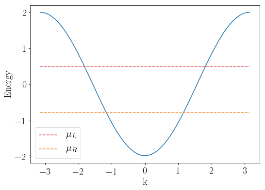
The electrons in both left and right leads have typical \(E(k) = 2(1 - \cos(k))\) tight binding dispersion. We plot the dispersion together with the chemical potentials \(\mu_{L/R}\):
kwant.plotter.bands(syst.leads[0], show=False)
plt.plot([-np.pi, np.pi], [mu_L] * 2, '--', color='#e15759', label=r"$\mu_L$")
plt.plot([-np.pi, np.pi], [mu_R] * 2, '--', color='#f28e2b', label=r"$\mu_R$")
plt.legend()
plt.show()
The leads can be defined using the \(\texttt{tkwant.manybody.lead_occupation}\) function in complete analogy to the standard Tkwant manybody wavefunction calculation. Here we set the left and right lead to have the chemical potentials \(\mu_L\) and \(\mu_R\):
occupations = [tkwant.manybody.lead_occupation(chemical_potential=mu_L),
               tkwant.manybody.lead_occupation(chemical_potential=mu_R)]
Without further specification, zero temperature is assumed in above case.
Time evolution and evaluation
The Tkwant class to calculate 2-time Green functions of different kind between two sites \(i\) and \(j\) is called \(\texttt{tkwant.manybody.GreenFunction}\). It is instatiated as:
green = tkwant.manybody.GreenFunction(syst, max(times), occupations)
The class \(\texttt{GreenFunction}\) uses the indexing of Kwant for the different lattice sites. While a lattice site is attributed by the user during the definition of the Hamiltonian, its index (which is an integer number) is an a priori arbitrary internal numbering from Kwant.
To show the difference between the site and its corresponding index, consider the definition of the Hamiltonian in this example. There, the left impurity has been attributed to the lattice site 0 (see line \(\texttt{syst[lat(0)] = eps_L}\) in function \(\texttt{make_double_impurity_system()}\)), but the actual index for this site is 1. While the indexing is still comprehensible in this simple example (the index increases from left to right, starting at the leftmost site with index 0), the situation gets more involved for extended and multiorbital systems.
Tkwant therefore provides the class \(\texttt{siteId}\) to easily obtain the correct index. An instance of \(\texttt{siteId}\) can be called with a lattice site to get the index in the Kwant ordering. Below we show how the index of the site with the left impurity can be obtained with the help of \(\texttt{siteId}\):
idx = tkwant.system.siteId(syst, lat)
site_0 = idx(0)
print('the left impurity has index= {} in the Kwant system'.format(site_0))
the left impurity has index= 1 in the Kwant system
The Green function can now be evolved forward in time with the \(\texttt{evolve()}\) method. Note that the \(\texttt{GreenFunction.evolve()}\) method takes 2 time arguments, in contrast to the similar method in the wave function objects that take only a single time argument. The \(\texttt{tkwant.manybody.GreenFunction}\) class provides also a \(\texttt{refine_intervals()}\) method, which should be called to ensure that the result is numerically correct. There is no evaluate method as for the wave function, but a method for each Green function type, which has to be called with two indices (obtained from \(\texttt{siteId}\)), referring to the corresponding lattice sites. Here we call the \(\texttt{lesser()}\) and the \(\texttt{retarded()}\) methods with \(i = j\) both on the lattice site 0 (left impurity position) to evaluate \(G_{00}^<\) and \(G_{00}^R\):
green_lesser = []
green_retard = []

for time in times:

    green.evolve(time, 0)
    green.refine_intervals()

    green_lesser.append(green.lesser(site_0, site_0))
    green_retard.append(green.retarded(site_0, site_0))
In the next step we calculate the referenc data.
Comparison to the analytical solution
The Green functions for the quantum dot array in flatband approximations are given in Eqs. (25), (28) and (32) and are implemented as special purpose routine in \(\texttt{tkwant.special.GreenFlatBand}\). For convenience, we have written the routine \(\texttt{make_double_impurity_matrices}\) to prepare the relevant input for our double dot system:
def make_double_impurity_matrices(gamma_L, gamma_C, gamma_R, epsilon_L, epsilon_R, mu_L, mu_R):
    h_ss = np.array([[epsilon_L, -gamma_C], [-gamma_C, epsilon_R]])
    h_se = np.array([[- gamma_L, 0], [0, - gamma_R]])
    gr_e = np.array([tkwant.special.g_ee_retarded(mu_L), tkwant.special.g_ee_retarded(mu_R)])
    mu_e = [mu_L, mu_R]
    return h_ss, h_se, gr_e, mu_e
From this, we can directly calculate \(G_{00}^<\) and \(G_{00}^R\) in flatband approximation:
matr = make_double_impurity_matrices(gamma_L, gamma_C, gamma_R, epsilon_L, epsilon_R, mu_L, mu_R)

green_flatband = tkwant.special.GreenFlatBand(*matr)

times_fine = np.linspace(0, 20, 201)
green_lesser_ref = np.array([green_flatband.lesser(0, 0, t) for t in times_fine])
green_retard_ref = np.array([green_flatband.retarded(0, 0, t) for t in times_fine])
We finally plot the Tkwant and the flatband results to see that they agree nicely:
green_lesser = np.array(green_lesser)
green_retard = np.array(green_retard)

fig, axes = plt.subplots(2, 2)
fig.set_size_inches(16, 10)

axes[0][0].plot(times_fine, green_lesser_ref.real, label='flatband')
axes[0][0].plot(times, green_lesser.real, 'o', label='Tkwant')
axes[0][0].set_title(r'$\Re G_{00}^<(t)$')

axes[0][1].plot(times_fine, green_lesser_ref.imag, label='flatband')
axes[0][1].plot(times, green_lesser.imag, 'o', label='Tkwant')
axes[0][1].set_title(r'$\Im G_{00}^<(t)$')

axes[1][0].plot(times_fine, green_retard_ref.real, label='flatband')
axes[1][0].plot(times, green_retard.real, 'o', label='Tkwant')
axes[1][0].set_title(r'$\Re G_{00}^R(t)$')

axes[1][1].plot(times_fine, green_retard_ref.imag, label='flatband')
axes[1][1].plot(times, green_retard.imag, 'o', label='Tkwant')
axes[1][1].set_title(r'$\Im G_{00}^R(t)$')


for axs in axes:
    for ax in axs:
        ax.set_xlabel(r'time $t$')
        ax.set_xlim(0, max(times))

plt.suptitle('$\gamma_L={}, \gamma_C={}, \gamma_R={}, \epsilon_L={}, \epsilon_R={}, \mu_L={}, \mu_R={}$'.
             format(gamma_L, gamma_C, gamma_R, epsilon_L, epsilon_R, mu_L, mu_R), size=22)

plt.subplots_adjust(wspace=0.3, hspace=0.4)
plt.legend(bbox_to_anchor=(1.1, 2.9))
plt.show()
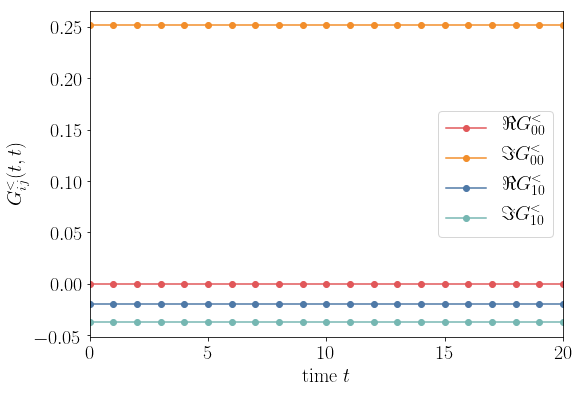
Calculating equal time diagonal and off-diagonal Green functions related to density and current
We write the discrete continuity equation in the form
where \(n_{i} = \langle c^\dagger_i(t) c_i(t) \rangle\) is the density on site \(i\) and \(I_{ij} = - I_{ji}\) the current flowing from site \(j\) to site \(i\). For a quadratic Hamiltonian as Eq. (1), we can derive the current (in units of \(\hbar\)) as
To calculate the onsite density and the current, they can be expressed in terms of the equal time \(G^<\) function Eq. (2):
Alternatively, both observables can be calculated using the wave function approach [2, 3] with
In the following we compute the density on the left (site 0) impurity \(n_0(t) = - i G^<_{00}(t,t)\) and the current \(I_{10}(t)\) from the left to the right impurity (site 0 to site 1) with the Green and the wave function approach. Our Hamiltonian matrix is static and with \(H_{10}(t) = - \gamma_C\) one finds \(I_{10}(t) = - 2 \gamma_C \Re G^<_{10}(t,t)\). First we compute the equal time Green functions to check that they are indeed constant in time:
green = tkwant.manybody.GreenFunction(syst, tmax=max(times), occupations=occupations)

g_less_00 = []
g_less_10 = []

idx = tkwant.system.siteId(syst, lat)
site_0 = idx(0)
site_1 = idx(1)

for time in times:

    green.evolve(time, time)
    green.refine_intervals()

    g_less_00.append(green.lesser(site_0, site_0))
    g_less_10.append(green.lesser(site_1, site_0))

g_less_00 = np.array(g_less_00)
g_less_10 = np.array(g_less_10)

plt.plot(times, g_less_00.real, 'o-', color='#e15759', label='$\Re G^<_{00}$')
plt.plot(times, g_less_00.imag, 'o-',color='#f28e2b', label='$\Im G^<_{00}$')

plt.plot(times, g_less_10.real, 'o-', color='#4e79a7', label='$\Re G^<_{10}$')
plt.plot(times, g_less_10.imag, 'o-', color='#76b7b2', label='$\Im G^<_{10}$')

plt.xlabel(r'time $t$')
plt.ylabel(r'$G^<_{ij}(t, t)$')
plt.xlim(0, max(times))
plt.legend()
plt.show()
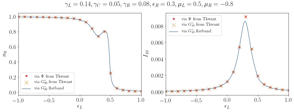
The stationary density and current can be obtained at initial time. Plotting the stationary density and current as function of Hamiltonian parameter \(\epsilon_L\) one can check that the Green and the wave function approach agree and the result also fits with the analytical flat band estimate.
n0_wave = []
n0_green = []
n0_flat = []

i10_wave = []
i10_green = []
i10_flat = []

epsilons = np.linspace(-1, 1, 21)

for epsilon_L_ in epsilons:

    syst, lat = make_double_impurity_system(gamma_L, gamma_C, gamma_R, epsilon_L_, epsilon_R)
    syst = syst.finalized()

    occupations = [tkwant.manybody.lead_occupation(chemical_potential=mu_L),
                   tkwant.manybody.lead_occupation(chemical_potential=mu_R)]

    # -- via wavefunction and density operator

    density_operator = kwant.operator.Density(syst, where=[lat(0)])
    current_operator = kwant.operator.Current(syst, where=[(lat(1), lat(0))])

    state = tkwant.manybody.State(syst, tmax=1, occupations=occupations)
    density = state.evaluate(density_operator)
    current = state.evaluate(current_operator)
    n0_wave.append(density)
    i10_wave.append(current)

    # -- via greenfunction from tkwant

    idx = tkwant.system.siteId(syst, lat)
    site_0 = idx(0)
    site_1 = idx(1)

    green = tkwant.manybody.GreenFunction(syst, tmax=1, occupations=occupations)
    g_less_00 = green.lesser(site_0, site_0)
    g_less_10 = green.lesser(site_1, site_0)

    density = g_less_00.imag
    current = - 2 * gamma_C * g_less_10.real
    n0_green.append(density)
    i10_green.append(current)

epsilons_fine = np.linspace(-1, 1, 201)

for epsilon_L_ in epsilons_fine:

     # -- via greenfunction in flatband approximation

    matr = make_double_impurity_matrices(gamma_L, gamma_C, gamma_R, epsilon_L_, epsilon_R, mu_L, mu_R)

    green_flatband = tkwant.special.GreenFlatBand(*matr)
    g_less_00 = green_flatband.lesser(0, 0, 0.)
    g_less_10 = green_flatband.lesser(1, 0, 0.)

    density = g_less_00.imag
    current = - 2 * gamma_C * g_less_10.real
    n0_flat.append(density)
    i10_flat.append(current)

#--- plot the results

fig, axes = plt.subplots(1, 2)
fig.set_size_inches(16, 5)

axes[0].plot(epsilons, n0_wave, 'o', color='#e15759', label='via $\Psi$ from Tkwant')
axes[0].plot(epsilons, n0_green, 'x', color='#f28e2b', markersize=12, label='via $G^<_{00}$ from Tkwant')
axes[0].plot(epsilons_fine, n0_flat, color='#4e79a7', label='via $G^<_{00}$ flatband')
axes[0].set_ylabel(r'$n_0$')

axes[1].plot(epsilons, i10_wave, 'o', color='#e15759', label='via $\Psi$ from Tkwant')
axes[1].plot(epsilons, i10_green, 'x', color='#f28e2b', markersize=12, label='via $G^<_{10}$ from Tkwant')
axes[1].plot(epsilons_fine, i10_flat, color='#4e79a7', label='via $G^<_{10}$ flatband')
axes[1].set_ylabel(r'$I_{10}$')

for ax in axes:
    ax.legend(fontsize=14)
    ax.set_xlabel(r'$\epsilon_L$')
    ax.set_xlim(min(epsilons), max(epsilons))

plt.suptitle('$\gamma_L={}, \gamma_C={}, \gamma_R={}, \epsilon_R={}, \mu_L={}, \mu_R={}$'.
             format(gamma_L, gamma_C, gamma_R, epsilon_R, mu_L, mu_R), size=22)

plt.show()
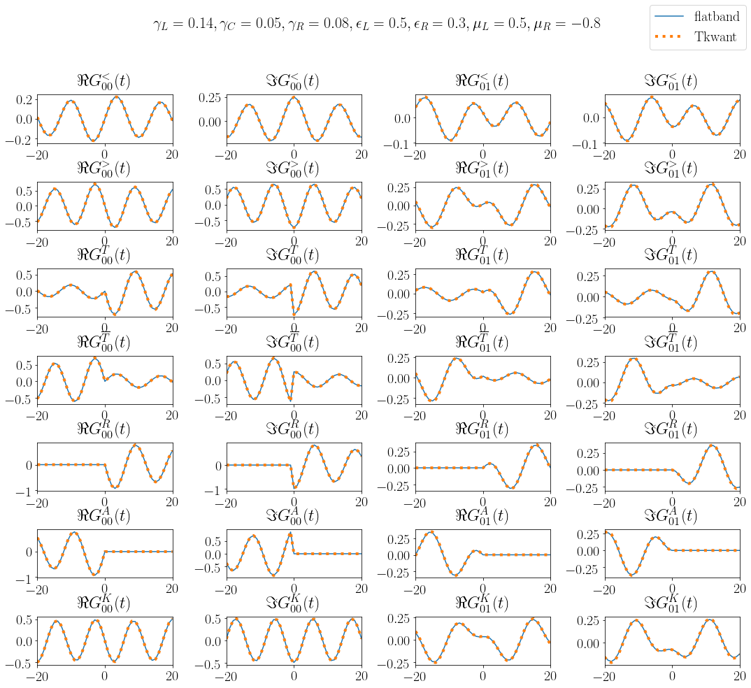
Various kinds of Green functions
Several kinds of nonequilibrium Greenfunctions can be defined. In the so-called contour base, one usually works with the lesser \(G^<\), greater \(G^>\), time-ordered \(G^T\) and anti-time ordered, \(G^{\bar{T}}\) whereas in the RAK basis, one usually works with the retarded \(G^{R}\), advanced \(G^{A}\) and the Keldysh \(G^{K}\) Green functions, see e.g. Ref. [1]. For Fermions, these Green functions are defined as
In above equations, \(T\) stands for the time-ordering and \(\bar{T}\) for the anti-time ordering operator. The class \(\texttt{tkwant.manybody.GreenFunction}\) has implemented all above Green functions. In the following we compute the different kind of Green functions for the diagonal \(G_{00}\) and the off-diagonal \(G_{01}\) elements.
green_types = {}
green_types['lesser'] = 'G^<'
green_types['greater'] = 'G^>'
green_types['ordered'] = 'G^T'
green_types['anti_ordered'] = 'G^{\overline{T}}'
green_types['retarded'] = 'G^R'
green_types['advanced'] = 'G^A'
green_types['keldysh'] = 'G^K'

green_data_00 = {key: [] for key in green_types.keys()}
green_data_01 = {key: [] for key in green_types.keys()}

syst, lat = make_double_impurity_system(gamma_L, gamma_C, gamma_R, epsilon_L, epsilon_R)
syst = syst.finalized()

# -- negative times
green = tkwant.manybody.GreenFunction(syst, max(times), occupations)

for time in times[1:]:
    green.evolve(0, time)
    green.refine_intervals()

    for gtype in green_types.keys():
        green_data_00[gtype].insert(0, getattr(green, gtype)(site_0, site_0))
        green_data_01[gtype].insert(0, getattr(green, gtype)(site_0, site_1))

# -- positive times
green = tkwant.manybody.GreenFunction(syst, max(times), occupations)

for time in times:
    green.evolve(time, 0)
    green.refine_intervals()

    for gtype in green_types.keys():
        green_data_00[gtype].append(getattr(green, gtype)(site_0, site_0))
        green_data_01[gtype].append(getattr(green, gtype)(site_0, site_1))

times_pm = np.concatenate((-times[:0:-1], times))
green_data_00 = {key: np.array(val) for key, val in green_data_00.items()}
green_data_01 = {key: np.array(val) for key, val in green_data_01.items()}
Note that we have splitted the above evolution in two parts to account for the positive and the negative time arguments as in Eqs. (5) and (6). The different kind of Green functions are computed also in flatband approximation:
matr = make_double_impurity_matrices(gamma_L, gamma_C, gamma_R, epsilon_L, epsilon_R, mu_L, mu_R)

green_flatband = tkwant.special.GreenFlatBand(*matr)

green_data_00_ref = {key: np.array([getattr(green_flatband, key)(0, 0, t) for t in times_pm])
                     for key in green_types.keys()}
green_data_01_ref = {key: np.array([getattr(green_flatband, key)(0, 1, t) for t in times_pm])
                     for key in green_types.keys()}
We find perfect agreement the numerical Tkwant result and the analytical flatband reference:
fig, axes = plt.subplots(len(green_types), 4)
fig.set_size_inches(18, 15)

for i, (key, gtype) in enumerate(green_types.items()):

    axes[i][0].plot(times_pm, green_data_00_ref[key].real, label='flatband')
    axes[i][0].plot(times_pm, green_data_00[key].real, linestyle='dotted', lw=4, label='Tkwant')
    axes[i][0].set_title('$\Re ' + gtype + '_{00}(t)$')

    axes[i][1].plot(times_pm, green_data_00_ref[key].imag, label='flatband')
    axes[i][1].plot(times_pm, green_data_00[key].imag, linestyle='dotted', lw=4, label='Tkwant')
    axes[i][1].set_title('$\Im ' + gtype + '_{00}(t)$')

    axes[i][2].plot(times_pm, green_data_01_ref[key].real, label='flatband')
    axes[i][2].plot(times_pm, green_data_01[key].real, linestyle='dotted', lw=4, label='Tkwant')
    axes[i][2].set_title('$\Re ' + gtype + '_{01}(t)$')

    axes[i][3].plot(times_pm, green_data_01_ref[key].imag, label='flatband')
    axes[i][3].plot(times_pm, green_data_01[key].imag, linestyle='dotted', lw=4, label='Tkwant')
    axes[i][3].set_title('$\Im ' + gtype + '_{01}(t)$')

for axx in axes:
    for ax in axx:
        ax.set_xlim(-max(times), max(times))

plt.suptitle('$\gamma_L={}, \gamma_C={}, \gamma_R={}, \epsilon_L={}, \epsilon_R={}, \mu_L={}, \mu_R={}$'.
             format(gamma_L, gamma_C, gamma_R, epsilon_L, epsilon_R, mu_L, mu_R), size=22)

plt.subplots_adjust(wspace=0.4, hspace=0.8)
plt.legend(bbox_to_anchor=(1.1, 13.8))

plt.show()
2.7.4. Example II: Single impurity site: quench of the coupling to the leads
Transient dynamics
To evaluate Greenfunctions also in the transient regime, we consider a single impurity model where the initially empty dot is connected at initial time \(t=0\) abruptly to the leads. The Hamiltonian is
with index \(0\) at the central impurity site. The hoppings \(\gamma_i(t) = 1\) for all \(i\), except at the impurity where \(\gamma_{-1}(t) = \gamma_{0}(t) = \gamma\theta(t)\), where \(\theta(x)\) is the Heaviside stepfunction. We choose the convention \(\theta(0) = 0\), such that the dot is initially disconnected and empty. Moreover we consider the symmetric equilibrium case with \(\mu_L = \mu_R = 0\) and zero temperature in the leads, and focus on the regime of weak coupling \(\gamma \ll 1\) such that we can compare to flatband approximation. The detailed calculation of the flatband Green function in this regime is given in the Appendix. Introducing \(\Gamma = 2 \gamma^2\), the lesser Green function on the dot can be written as
Note that an almost identical expression has been derived in Ref. [6], except a typo as the oscillating factor \(e^{-i \epsilon_0 (t - t')}\) is missing in Eq. (15) of that reference. The occupation on the dot \(n(t)\) can be obtained again from the equal time \(G^<\) function via \(n(t) = - i G_{00}^<(t, t)\). The long-time limit corresponds to the stationary equilibrium density \(n_{eq}\) on the dot and one obtains the well-known relation
The Tkwant simulation for the Green function can be performed very similar to all examples above, except that the coupling between the lead and the dot are now time dependent. Due to the abrupte switching of the leads, the integrand over the different energy modes is getting numerically complicated and cause the adaptive integration routine to use many integral subdivisions. The simulation is therefore too time consuming for running this tutorial in real time. We will show therefore only the result, but provide the Python scripts to perform the simulation below.

Above simulations shows the lesser Green function with different (left) and identical (right) time arguments. The density \(n(t)\) on the dot is calculated with Tkwant using the manybody wave function approach. The value \(n_{eq}\) is computed from Tkwant using the manybody wave function approach for the stationary problem where lead couplings are time independent and \(n_{eq}\) in flatband approximation is obtained from Eq. (48). The parameters are \(\epsilon_0 = \gamma = 0.1\) and \(t_0 = 100\).
See also
The above figure can be obtained by running the two Python scripts:
2.7.5. References
[1] H. Haug and A. P. Jauho, Quantum Kinetics in Transport and Optics of Semiconductors 2nd ed. (Springer, Berlin, 2008).
[2] B. Gaury, J. Weston, M. Santin, M. Houzet, C. Groth, and X. Waintal, Numerical simulations of time-resolved quantum electronics Phys. Rep. 534, 1 (2014).
[3] T. Kloss, J. Weston, B. Gaury, B. Rossignol, C. Groth and X. Waintal, Tkwant: a software package for time-dependent quantum transport New J. Phys. 23, 023025 (2021).
[4] A.-P. Jauho, N. S. Wingreen, and Y. Meir, Time-dependent transport in interacting and noninteracting resonant-tunneling systems Phys. Rev. B 50, 5528 (1994).
[5] C. W. Groth, M. Wimmer, A. R. Akhmerov, and X. Waintal, Kwant: a software package for quantum transport New J. Phys. 16, 063065 (2014).
[6] R.-P. Riwar and T. L. Schmidt, Transient dynamics of a molecular quantum dot with a vibrational degree of freedom Phys. Rev. B 80,125109 (2009).
[7] Y. N. Fernández, M. Jeannin, P. T. Dumitrescu, T. Kloss, J. Kaye, O. Parcollet, and X. Waintal, Learning Feynman Diagrams with Tensor Trains Phys. Rev. X 12, 041018 (2022).
2.7.6. Appendix
Nonequilibrium Green functions in flatband approximationIn the following we derive zero temperature Green functions for a one dimensional quantum dot array in flatband approximation. The derivation is close to the one in Ref. [7], except that we calculate true nonequilibrium Green functions such that no fluctuation-dissipation theorem is present in the central system. The Green function is defined as
(15)¶\[\begin{equation} G^{-1} = (\omega - H). \end{equation}\]It is practical to write above equation in a block matrix form to separate into a finite central system (S) and to the environment (E) which represents the semi-infinite leads:
(16)¶\[\begin{split}\begin{equation} G^{-1} = \left( \begin{array}{cc} G_{SS}^{-1} & G_{SE}^{-1} \\ G_{ES}^{-1} & G_{EE}^{-1} \end{array} \right), \quad H = \left( \begin{array}{cc} H_{SS} & H_{SE} \\ H_{ES} & H_{EE} \end{array} \right). \end{equation}\end{split}\]Each of the Green function blocks with index \(\alpha, \beta \in \{S, E \}\) has again a Keldysh block structure
(17)¶\[\begin{split}\begin{equation} G_{\alpha \beta} = \left( \begin{array}{cc} G^R & G^K \\ & G^A \end{array} \right)_{\alpha \beta}, \quad G^{-1}_{\alpha \beta} = \left( \begin{array}{cc} (G^R)^{-1} & - (G^R)^{-1} G^K (G^A)^{-1} \\ & (G^A)^{-1} \end{array} \right)_{\alpha \beta}. \end{equation}\end{split}\]The separated system and environment Green functions can be obtaind from
(18)¶\[\begin{split}\begin{align} G_{SS}^{-1} &= \omega - H_{SS} - H_{SE} (\omega - H_{EE})^{-1} H_{ES},\\ G_{EE}^{-1} &= \omega - H_{EE}. \end{align}\end{split}\]We will now concentrate on the Green functions of the system. Using the Keldysh blockstructure one finds
(19)¶\[\begin{split}\begin{align} (G^R_{SS})^{-1} &= \omega - H_{SS} - H_{SE} G_{EE}^R H_{ES}, \\ (G^A_{SS})^{-1} &= \omega - H_{SS} - H_{SE} G_{EE}^A H_{ES}, \\ G^K_{SS} &= G^R_{SS} H_{SE} G_{EE}^K H_{ES} G^A_{SS}. \end{align}\end{split}\]To invert above equations, the effective Hamiltonian of the retarded Green function is written as
(20)¶\[\begin{equation} H_{SS} + H_{SE} G_{EE}^R H_{ES} = U D U^{-1}, \end{equation}\]where \(D\) is a diagonal matrix. We find
(21)¶\[\begin{split}\begin{align} G^R_{SS}(\omega) &= U (\omega - D)^{-1} U^{-1} , \\ G^A_{SS}(\omega) &= U^* (\omega - D^*)^{-1} (U^*)^{-1} , \\ G^K_{SS}(\omega) &= U (\omega - D)^{-1} U^{-1} H_{SE} G^K_{EE} H_{ES} U^* (\omega - D^*)^{-1} (U^*)^{-1}, \end{align}\end{split}\]where we have used that \(G^A(\omega) = (G^R(\omega))^*\). As the different leads are not coupled, all \(G^{\kappa}_{EE}\) with \(\kappa \in \{ R,A,K\}\) are diagonal matrices. One can therefore use the simplified notation
(22)¶\[\begin{equation} g^K_\alpha(\omega) \equiv [G^K_{EE}]_{\alpha \alpha} = (1 - 2 f_\alpha(\omega)) [g^R_\alpha - g^A_\alpha] \end{equation}\]for the components of the lead Green functions. We have also set \(g^{R/A}_\alpha(\omega) \approx g^{R/A}(\mu_\alpha) \equiv g^{R/A}_\alpha\), such that the lead Green functions are frequency independent. This is also known as flatband approximation. The Fermi function is
(23)¶\[\begin{equation} f_{\alpha}(\omega) = \frac{1}{1 + e^{(\omega - \mu_\alpha)/T_\alpha}}, \end{equation}\]where \(\mu_\alpha\) is the chemical potential and \(T_\alpha\) the temperature on lead \(\alpha\). Performing a Fourier transform to the time domaine
(24)¶\[\begin{equation} G(t) = \int_{-\infty}^{\infty} \frac{d \omega}{2 \pi} \, e^{- i \omega t} G(\omega) \end{equation}\]we find for the retarded and the advanced Green functions
(25)¶\[\begin{split}\begin{align} G^R_{SS}(t) &= (2 \pi)^{-1} U I(D, t) U^{-1} , \\ G^A_{SS}(t) &= (2 \pi)^{-1} U^* I(D^*, t) (U^*)^{-1} . \end{align}\end{split}\]Using contour integration, one finds the frequency integrals for \(\Im{a} \neq 0\), \(t \neq 0\) as
(26)¶\[\begin{split}\begin{equation} I(a, t) = \int_{-\infty}^{\infty} d \omega \, e^{- i \omega t} \frac{1}{\omega - a} = \begin{cases} - 2 \pi i \, \textrm{sgn}(t) e^{- i a t} \theta(- \Im a t) &\quad \Re{a} \neq 0 \\ - \pi i \, \textrm{sgn}(t) e^{- i a t} \theta(- \Im a t) &\quad \Re{a} = 0 . \end{cases} \end{equation}\end{split}\]To perform Fourier transform of the Keldysh Green function, we write matrix function component wise as (Einstein sum convention):
(27)¶\[\begin{equation} G^K_{ij}(\omega) = U_{il} (\omega - D)^{-1}_{l} U^{-1}_{lm} H^{SE}_{mn} g^K_{n}(\omega) H^{ES}_{nm'} U^*_{m'l'} (\omega - D^*)^{-1}_{l'} (U^*)^{-1}_{l'j}. \end{equation}\]In the time domaine, the Keldysh Green function is
(28)¶\[\begin{align} G^K_{ij}(t) = U_{il} U^{-1}_{lm} H^{SE}_{mn} (g^R_{n} - g^A_{n}) Q_{n}(D_l, D^*_{l'}, t) H^{ES}_{nm'} U^*_{m'l'} (U^*)^{-1}_{l'j} \end{align}\]with
(29)¶\[\begin{equation} Q_{n}(a, b, t) = \int_{-\infty}^{\infty} \frac{d \omega}{2 \pi} \, e^{- i \omega t} \frac{1 - 2 \theta(\mu_n - \omega)}{(\omega - a)(\omega - b)}. \end{equation}\]Note that we have taken the zero temperature limit \(T \rightarrow 0\) such that \(f_\alpha(\omega) = \theta(\mu_\alpha - \omega)\) in above expression. Doing the integral one finds for \(t \neq 0, \, a \neq b\)
(30)¶\[\begin{split}\begin{align} Q_{n}(a, b, t) &= \frac{1}{2 \pi (a - b)} \Bigl[ \int_{-\infty}^{\infty} d \omega \, \frac{e^{- i \omega t}}{\omega - a} - \int_{-\infty}^{\infty} d \omega \, \frac{e^{- i \omega t}}{\omega - b} - 2 \int_{-\infty}^{\mu_n} d \omega \, \frac{e^{- i \omega t}}{\omega - a} + 2 \int_{-\infty}^{\mu_n} d \omega \, \frac{e^{- i \omega t}}{\omega - b} \Bigr] \\ &= \frac{1}{2 \pi (a - b)} \Bigl[ I(a, t) - I(b, t) + 2 e^{- i \mu_n t} [I^<( a - \mu_n, t) - I^<(b - \mu_n, t) ] \Bigr], \quad \text{if } t \neq 0, \, a \neq b \\ I^<(a, t) &= - \int_{-\infty}^{0} d \omega \frac{e^{- i \omega t}}{\omega - a} \\ & = \begin{cases} e^{-i a t} \left[ E_1(-i a t) + 2 \pi i \, \textrm{sgn}(t) \theta(-\Im a t) \theta(-\Re a) \right] &\quad \Re{a} \neq 0 \\ e^{- i a t} [- E_i(i a t) + \pi i \, \textrm{sgn}(t) \theta[- \Im{at}]] &\quad \Re{a} = 0 \end{cases}, \quad \Im{a} \neq 0, t \neq 0 . \end{align}\end{split}\]The two exponential integrals are \(E_1(z) = \int_z^\infty dx \, e^{-x} / x\) for \(z \in \mathbb{C}\) with \(|\arg(z)| < \pi\) and \(E_i(x) = -\int_{-x}^\infty dt \, e^{-t} / t\) for real and non-zero \(x\). For \(t = 0\) one finds
(31)¶\[\begin{split}\begin{align} \int_{-\infty}^{\infty} d \omega \, \frac{1}{(\omega - a)(\omega - b)} &= \frac{2 \pi i}{a - b} \Bigl(\theta(\Im a) - \theta(\Im b) \Bigr) , \\ \int_{-\infty}^{\mu} d \omega \, \frac{1}{(\omega - a)(\omega - b)} &= \frac{\log(a - \mu) - \log(b - \mu)}{a - b}, \end{align}\end{split}\]such that
(32)¶\[\begin{align} Q_{n}(a, b, t=0) = \frac{1}{(a - b)} \Bigl[ i \left(\theta(\Im a) - \theta(\Im b) \right) - \frac{1}{\pi} \left(\log(a - \mu_n) - \log(b - \mu_n)\right) \Bigr] . \end{align}\]Having the three Keldysh Green functions, one can obtain the lesser and greater Green functions from the well-known relation
(33)¶\[\begin{split}\begin{align} G^< &= \frac{1}{2} \left( G^K - G^R + G^A \right) , \\ G^> &= \frac{1}{2} \left( G^K + G^R - G^A \right). \end{align}\end{split}\]Double quantum dot
For the Hamiltonian in Eq. (4) the Hamiltonian matrices are
(34)¶\[\begin{split}\begin{align} H_{SS} = \left( \begin{array}{cc} \epsilon_L & - \gamma_C \\ - \gamma_C & \epsilon_R \end{array} \right), \quad H_{SE} = H_{ES}^\dagger = \left( \begin{array}{cc} -\gamma_L & \\ & -\gamma_R \end{array} \right). \end{align}\end{split}\]The semi-infinite chain with couplings \(H_{i, i+i} = -1\) can be solved exactly and one finds
(35)¶\[\begin{equation} g^R(\omega) = \frac{\omega}{2} - i \sqrt{1 - \left(\frac{\omega}{2}\right)^2}, \quad \omega \in [-2, 2] \end{equation}\]with \(g^A(\omega) = (g^R(\omega))^*\). Note that \(g^R(\omega)\) corresponds to the lead self-energy in Eq. (C3) of Ref. [2].
Single quantum dot after suddenly coupling the leads
We will derive the lesser Green function \(G^<\) for a single quantum dot and initially empty quantum dot which is suddenly coupled to two semi-infinite leads. For simplicity we choose the coupling \(\gamma\) to both leads and also their chemical potential \(\mu\) identical. Moreover we will work at the small coupling limit such that one can again use flatband approximation. The derivation is close to the one in Ref. [6].
The Hamiltonian matrices for the Hamiltonian in Eq. (12) are
(36)¶\[\begin{split}\begin{align} H_{SS} = \epsilon_0, \quad H_{SE} = H_{ES}^\dagger = \left( \begin{array}{cc} -\gamma & \\ & -\gamma \end{array} \right). \end{align}\end{split}\]We choose \(\mu_{L/R} = 0\) such that \(g^R_{L/R}(0) = -i\). To simplify the notation, the dot Green function is written as \(G^\kappa \equiv [G^\kappa_{SS}]_{00}\). Retarded and advanced Green functions can be written in form of a Dyson equation
(37)¶\[\begin{align} G^{R/A} &= ( \omega - \epsilon_0 - \Sigma^{R/A})^{-1} \end{align}\]where the so-called lead self-energies are
(38)¶\[\begin{split}\begin{align} \Sigma^{R/A}(\omega) &= \mp i \Gamma, \\ \Sigma^K (\omega) &= 2 \gamma^2 g^K = -2 i \Gamma (1 - 2 f(\omega)), \\ \Sigma^< (\omega) &= \frac{1}{2} \left( \Sigma^K - \Sigma^R + \Sigma^A \right) = 2 i \Gamma f(\omega) \end{align}\end{split}\]where \(f\) is again the Fermi function and the effective coupling constant is \(\Gamma = 2 \gamma^2\). Note that we have also used the fluctuation-dissipation relation for the lead Green functions
(39)¶\[\begin{equation} g^K(\omega) = (1 - 2 f(\omega))(g^R(\omega) - g^A(\omega) ) = - 2 i (1 - 2 f(\omega)). \end{equation}\]The the time domaine, the Dyson equation for the retarded and the advanced Green function can be written as
(40)¶\[\begin{equation} G^{R/A}(t,t') = G^{R/A}_0(t - t') + \int_0^\infty \int_0^\infty dt_1 dt_2 G^{R/A}_0(t - t_1) \Sigma^{R/A}(t_1 - t_2) G^{R/A}(t_1,t') \end{equation}\]where the subscript 0 refers to the Green function without lead
(41)¶\[\begin{equation} G^{R/A}_0(t) = \mp i \theta(\pm t) e^{- i \epsilon_0 (t - t')}. \end{equation}\]and the self-energy in the time domaine is
(42)¶\[\begin{split}\begin{align} \Sigma^{R/A}(t) &= \mp i \Gamma \delta(t), \\ \Sigma^{<}(t) &= \frac{i \Gamma}{\pi} \int_{-\infty}^0 d \omega \, e^{- i \omega t}, \end{align}\end{split}\]where we have used again the zero temperature limit for \(\Sigma^{<}\). The full retarded and advanced Green with leads are
(43)¶\[\begin{align} G^{R/A}(t, t') &= \mp i \theta(\pm(t - t')) e^{- i \epsilon_0 (t - t') \mp \Gamma(t - t')} \end{align}\]and solve above Dyson equation. The lesser Green function can be written as an integral equation [1]:
(44)¶\[\begin{equation} G^< = (1 + G^R \Sigma^R) G^<_0 (1 + G^A \Sigma^A) + G^R \Sigma^< G^{A}. \end{equation}\]This form is practical for an initially empty dot as then the first term is zero. In our case, above equation takes the explicit form
(45)¶\[\begin{split}\begin{align} G^<(t, t') &= \int_0^\infty dt_1 \int_0^\infty dt_2 G^R_0(t - t_1) \Sigma^<(t_1 - t_2) G^A(t_1 - t') \\ &= \frac{i \Gamma}{\pi} e^{- i \epsilon_0 (t - t') - \Gamma(t + t')} \int_{-\infty}^0 d \omega \int_0^t dt_1 \int_0^{t'} dt_2 e^{- i (\omega - \epsilon_0) t + \Gamma t} e^{i (\omega - \epsilon_0) t' + \Gamma t'}. \end{align}\end{split}\]After integrating over \(t_1\) and \(t_2\) one finds
(46)¶\[\begin{align} G^<(t, t') = \theta(t) \theta(t') \frac{i \Gamma}{\pi} e^{-i \epsilon_0 (t - t')} \int_{-\infty}^0 d \omega \frac{1}{(\omega - \epsilon_0)^2 + \Gamma^2} \left( e^{-i (\omega - \epsilon_0) t} - e^{- \Gamma t}\right) \left( e^{i (\omega - \epsilon_0) t'} - e^{- \Gamma t'}\right). \end{align}\]As mentioned before, this form is basically equivalent to Eq. (15) in Ref. [6], except of the oscillating factor \(e^{-i \epsilon_0 (t - t')}\) which is missing in that reference. One can perform the remaining frequency integral via contour integration to finally obtain
(47)¶\[\begin{split}G^<(t, t') &= \theta(t) \theta(t') \frac{1}{2 \pi} \Bigl[ I^<(\epsilon_0 - i \Gamma, t - t') - I^<(\epsilon_0 + i \Gamma, t - t') + 2 \pi i n_{eq} e^{-i \epsilon_0 (t - t') - \Gamma (t + t')} \\ & \qquad \quad \quad \quad - e^{i \epsilon_0 t' - \Gamma t'} \left[I^<(\epsilon_0 - i \Gamma, t) - I^<(\epsilon_0 + i \Gamma, t)\right] \\ & \qquad \quad \quad \quad - e^{-i \epsilon_0 t - \Gamma t} \left[I^<(\epsilon_0 - i \Gamma, -t') - I^<(\epsilon_0 + i \Gamma, -t')\right] \Bigr] , \\ G^<(t, t) &= \theta(t) \Bigl[ i n_{eq} \left(1 + e^{- 2 \Gamma t} \right) - \frac{e^{- \Gamma t}}{2 \pi} \bigl(e^{i \epsilon_0 t} \left[I^<(\epsilon_0 - i \Gamma, t) - I^<(\epsilon_0 + i \Gamma, t) \right] \\ &\qquad \quad - e^{-i \epsilon_0 t} \left[ I^<(\epsilon_0 - i \Gamma, -t) - I^<(\epsilon_0 + i \Gamma, -t) \right] \bigr) \Bigr],\end{split}\]with
(48)¶\[\begin{equation} n_{eq} = \frac{\Gamma}{\pi}\int_{-\infty}^0 d \omega \frac{1}{(\omega - \epsilon_0)^2 + \Gamma^2} = \frac{1}{\pi} \arctan \left(-\frac{ \epsilon_0}{\Gamma} \right) + \frac{1}{2}. \end{equation}\]